Documentation Revision Date: 2026-05-29
Dataset Version: 1
Summary
This dataset contains 29 data files: 14 files in comma-separated (CSV) format and 15 in cloud-optimized GeoTIFFs.
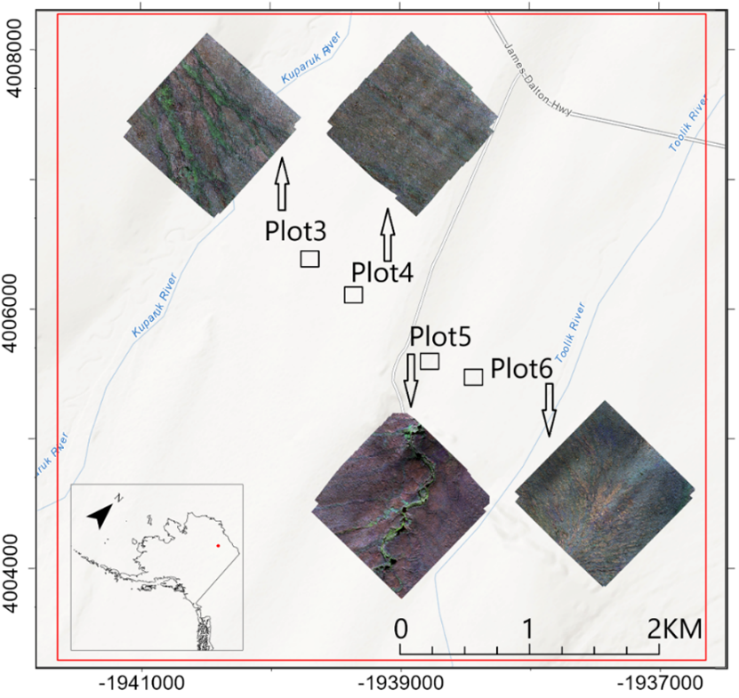
Figure 1. The study region within the Arctic foothills tundra around Imnavait Creek, Alaska (lat 68.6167, lon -149.3167; red dot in the inset map). The region consists of five intensively sampled plots (Plot_2, Plot_3, Plot_4, Plot_5, and Plot_6; 90 m x 90 m each; black rectangles) with their corresponding RGB (red-green-blue) composite drone images displayed alongside. Plot_2 is not shown in this Figure. Plot_1 was not sampled in this field campaign. Adapted from Du et al (2025).
Citation
Bakian-Dogaheh, K., J. Du, K.A. Endsley, J. Kim, R. De Sobrino, J.N. Tapia, R. Fulweber, A.B. Young, J.S. Kimball, and M. Moghaddam. 2026. ABoVE: Active Layer Soil Properties and Multispectral Images, Imnavait Creek AK, 2024. ORNL DAAC, Oak Ridge, Tennessee, USA. https://doi.org/10.3334/ORNLDAAC/2473
Table of Contents
- Dataset Overview
- Data Characteristics
- Application and Derivation
- Quality Assessment
- Data Acquisition, Materials, and Methods
- Data Access
- References
Dataset Overview
This dataset provides active layer soil properties measurements and multi-spectral Unmanned Aerial Vehicle (UAV)-based imagery from Imnavait Creek, Alaska, USA in 2024 in support of the NASA Arctic and Boreal Vulnerability Experiment (ABoVE) Airborne Campaign. Soil properties include active layer thickness, soil roughness height, soil organic matter, bulk density, root biomass, soil carbon and nitrogen, and mineral texture. Soil samples were collected from the top 30 cm from 2024-08-17 to 2024-08-23. A DJI Matrice 210 v2 UAV was flown on 2024-09-04 to collect optical (RGB) images, optical derived digital surface model (DSM), and multispectral images. Normalized difference vegetation index (NDVI) was calculated from multispectral images. This dataset provides a unique, comprehensive, and simultaneous characterization of the active layer, supporting analyses of fine scale heterogeneity of soil processes in the active layer in areas over permafrost and the drivers that influence topsoil organic matter in Arctic foothills tundra.
Project: Arctic-Boreal Vulnerability Experiment
The Arctic-Boreal Vulnerability Experiment (ABoVE) was a field campaign conducted in Alaska and western Canada for nearly ten years, starting in 2015. Researchers participating in ABoVE linked field-based, process-level studies with geospatial data products derived from airborne and satellite sensors. The work provided a foundation for improving the analysis and modeling capabilities needed to understand and predict ecosystem responses to, and societal implications of, climate change in the Arctic and boreal regions.
Related Publication:
Du, J., K.A. Endsley, K. Bakian-Dogaheh, J. Kimball, M. Moghaddam, T. Douglas, A. Melebari, S. Eskandari, J. Kim, J. Whitcomb, Y. Zhao, and S. Henze. 2025. Assessing spatial heterogeneity of active layer thickness over Arctic-foothills tundra through intensive field sampling and multi-source remote sensing. EGUsphere (preprint). https://doi.org/10.5194/egusphere-2025-3236
Related Datasets:
Bakian-Dogaheh, K., R.H. Chen, M. Moghaddam, Y. Yi, and A. Tabatabaeenejad. 2020. ABoVE: Active Layer Soil Characterization of Permafrost Sites, Northern Alaska, 2018. ORNL DAAC, Oak Ridge, Tennessee, USA. https://doi.org/10.3334/ORNLDAAC/1759
Bakian-Dogaheh, K., R.H. Chen, Y. Yi, T.D. Sullivan, R.J. Michaelides, A.D. Parsekian, K. Schaefer, A. Tabatabaeenejad, J. Kimball, and M. Moghaddam. 2023. Soil Matric Potential, Dielectric, and Physical Properties, Arctic Alaska, 2018. ORNL DAAC, Oak Ridge, Tennessee, USA. https://doi.org/10.3334/ORNLDAAC/2149
Acknowledgments
Funding was provided by the Arctic Boreal Vulnerability Experiment (ABoVE) of the NASA Terrestrial Ecology program (grant 80NSSC22K1238, ABoVE Phase 3). The Toolik Field Station funding was provided by the National Science Foundation (NSF) Cooperative Agreement: Toolik Field Station Base Funding (award 2221133, 2022-2027).
Data Characteristics
Spatial Coverage: Imnavait Creek Watershed, Northern Alaska, USA
ABoVE Reference Locations: Domain: Core ABoVE, State/territory: Alaska, Grid cell: Ah1v0Bh8v3Ch48v21
Spatial Resolution: Field measurements: point locations, Imagery and DSM: 0.7 to 2.7 cm
Temporal Coverage: Field measurements: 2024-08-17 to 2024-08-23, UAV imagery: 2024-09-04
Temporal Resolution: One-time measurements.
Study Area: Latitude and longitude are given in decimal degrees.
| Site | Westernmost Longitude | Easternmost Longitude | Northernmost Latitude | Southernmost Latitude |
|---|---|---|---|---|
| Imnavait Creek, Alaska | -149.37 | -149.31 | 68.63 | 68.62 |
Data File Information
This dataset contains 29 data files: 14 files in comma-separated values format (*.csv) and 15 cloud-optimized GeoTIFFs (*.tif).
CSV files
These files hold field measurements and soil characteristics. The naming convention is <variable>_Plot_<plotnum>.csv, where
- <variable> is the measured variable: "ALT" = active layer thickness, "ROUGHNESS" = soil roughness, "SOIL" = soil biogeochemical and physical properties. See Tables 1-3 for variable descriptions.
- <plotnum> is the plot number 2 to 6.
Missing data is indicated by "NA" for string variables and -9999 for numeric variables.
GeoTIFF files
The file naming convention is <imagery>_Plot_<plotnum>.tif, where
- <imagery> is the UAV imagery product: "RGB" = Red-Blue-Green) imagery using a DJI x7 24mm lens, "DSM" = surface elevation (including vegetation and other structures on the landscape) in m, and "MULTISPECTRAL" = multispectral imagery collected using the Micasense Red-Edge MX sensor at 2.7-cm resolution.
GeoTIFF characteristics
- Coordinate system: UTM zone 6N, NAD83(2011) datum; EPSG 6335
- Spatial resolution: 0.7 cm (RGB), 1.2 cm (DSM), or 2.7 cm (MULTISPECTRAL)
- Bands: three (RGB), one (DSM), or six (MULTISPECTRAL, Table 4)
- Nodata value: -9999 for DSM and MULTISPECTRAL
- Data type: Byte for RGB; Float32 for DSM and MULTISPECTRAL
Table 1. Data dictionary for ALT_Plot_#.csv files, including measurements of active layer thichness (ALT).
| Variable | Units | Description |
|---|---|---|
| ALT_ID | - | ALT measurement ID in ALT-<A>-<B> format where <A> is the plot number and <B> is the grid location (Figure 3). |
| X | m | X coordinate in Canada_Albers_Equal_Area_Conic (ESRI:102001) |
| Y | m | Y coordinate in Canada_Albers_Equal_Area_Conic (ESRI:102001) |
| Latitude | degrees north | Latitude in decimal degrees of the sampling point |
| Longitude | degrees east | Longitude in decimal degrees of the sampling point |
| ALT-1 | inch | First ALT measurement in inches |
| ALT-2 | inch | Second ALT measurement in inches |
| ALT-3 | inch | Third ALT measurement in inches |
| ALT-1_cm | cm | First ALT measurement in cm |
| ALT-2_cm | cm | Second ALT measurement in cm |
| ALT-3_cm | cm | Third ALT measurement in cm |
| AVG | cm | Average ALT for all 3 points in cm |
| Group | - | Grouping based on same X values, and increment or decrement of the Y (17 sampling points in each group) |
| Water | - | Presence of water: "S1" = Saturated but little/no standing water; "S2" = Standing water (kettle pond); and "S3" = Creek or stream |
| Notes | - | Notes about vegetation or presence of rock |
| Soil_Core_ID | - | Corresponding Soil Core ID |
Table 2. Data dictionary for ROUGHNESS_Plot_#.csv files.
| Variable | Units | Description |
|---|---|---|
| ROUGHNESS_ID | - | Roughness ID in Roughness-<A>-<B>-<C>-<D> format where <A> is the plot number, <B> is subplot, <C> is the sub-subplot number, and <D> is the point number along the transect (1-51) (e.g., "Roughness-2-1-1-3"). See Figure 3. |
| X | m | X coordinate in Canada_Albers_Equal_Area_Conic (ESRI:102001) |
| Y | m | Y coordinate in Canada_Albers_Equal_Area_Conic (ESRI:102001) |
| Latitude | degrees north | Latitude in decimal degrees of the sampling subplot center |
| Longitude | decimal east | Longitude in decimal degrees of the sampling subplot center |
| Length | cm | Refers to the length from center of a 100 cm tape measure attached to the spirit level |
| South-to-North Height | m | Measured height from a laser altimeter, when the direction of the tape measure is south-to-north. |
| East-to-West Height | m | Measured height from a laser altimeter, when the direction of the tape measure is east-to-west. |
Table 3. Data dictionary for SOIL_Plot_#.csv files.
| Variable | Units | Description |
|---|---|---|
| SOIL_ID | - | Soil ID in Soil-A-B-C-D format where A is the plot number, B is subplot, C is the sub-subplot number, and D is the sample number (1-6). See Figure 3. |
| X | m | X coordinate in Canada_Albers_Equal_Area_Conic (ESRI:102001) |
| Y | m | Y coordinate in Canada_Albers_Equal_Area_Conic (ESRI:102001) |
| latitude | degrees north | Latitude in decimal degrees of the sampling point |
| longitude | degrees east | Longitude in decimal degrees of the site |
| sampling_date | YYYY-MM-DD | Date samples were collected |
| hour | HH:mm | Time in in hour:minute (00:00-23:59) format, local Alaska time |
| min_depth | cm | Minimum sampling depth |
| max_depth | cm | Maximum sampling depth |
| avg_depth | cm | Average of min and max depth |
| soil_moisture | cm3 cm-3 | Volumetric soil moisture of the soil sample in the field (total sample’s soil moisture) |
| field_bulk_density | g cm-3 | Bulk density of the soil sample in the field (total bulk density) |
| root_biomass | (g g-1)*100 | Gravimetric fraction of the sample’s coarse organic matter (live and dead fine roots) with dimension >2 mm over the entire dry sample, referred to as root biomass (RB); recorded as percent |
| gravel_fraction | (g g-1)*100 | Gravimetric fraction of mineral particles (gravels) with size >2 mm over the total dry sample weight, referred to as gravel fraction (GF); recorded as percent |
| organic_matter | (g g-1)*100 | Total organic matter in the sample. OM=RB + SOM x (1- RB/100 - GF/100) |
| soil_organic_matter | (g g-1)*100 | Gravimetric fraction of the soil organic matter with dimension <2 mm over the fraction of dry sample with dimension <2 mm (knowingly as soil). Measured by loss on ignition; recorded as percent |
| soil_carbon | (g g-1)*100 | Percentage of soil carbon is measured by CHN elemental analyzer method using high temperature combustion. No acidification treatment was done to remove inorganic carbon; recorded as percent |
| soil_nitrogen | ppm | Part per million of soil nitrogen measured by combustion method |
| sand | (g g-1)*100 | Gravimetric fraction of the sand content over the fraction of dry soil sample with dimension <2 mm (knowingly as soil), measured by hydrometer method, without removal of organic matter; recorded as percent |
| silt | (g g-1)*100 | Soil silt fraction in percent |
| clay | (g g-1)*100 | Soil clay fraction in percent |
| soil_type | - | Type of mineral soil according to soil classification |
Table 4. Band descriptions for MULTISPECTRAL_Plot_#.tif files.
| Bands | Description | Center Wavelength (nm) | Bandwidth (nm) |
|---|---|---|---|
| Band 1 | Blue | 475 | 32 |
| Band 2 | Green | 560 | 27 |
| Band 3 | Red | 668 | 14 |
| Band 4 | Red edge | 717 | 12 |
| Band 5 | Near-IR | 842 | 57 |
| Band 6 | Normalized Difference Vegetation Index | - | - |
Application and Derivation
Active layer thickness (ALT) is a key indicator of permafrost degradation and is primarily important to understand the main drivers of permafrost thaw and ALT deepening, and associated variability at different scales. Soil biogeochemical properties such as soil organic matter, root biomass, and other soil physical properties are primarily important for parameterization of ecosystem models to study the dynamics of the permafrost active layer under the regional warming trends in the Arctic. Along with soil roughness height, this information is also critical for inclusion in physics-based, computational radar remote sensing models that map the carbon and subsurface water characteristics of active layers using radar backscatter. UAV imagery is key in providing a foundational dataset that bridges the observational gap between detailed field measurements and coarser footprint retrievals obtained from airborne and satellite remote sensing, and regional process models. UAV-based multi-spectral and optical imagery provides detailed local information on vegetation structure and microtopography that is immensely beneficial for delineating micro-scale (centimeters level resolution) heterogeneity of the permafrost landscape.
This dataset provides a unique, comprehensive, and simultaneous characterization of basic soil properties, soil roughness height, active layer thickness, and multispectral UAV imagery in support of the NASA Arctic and Boreal Vulnerability Experiment (ABoVE) Airborne Campaign (AAC). The site locations were carefully selected to capture different landscapes within a key benchmark AAC flight line known as Toolik. An additional L-band SAR airborne (UAVSAR) flight was requested to sample the Toolik AAC flight line in a forward/backward direction (toolik_23315 and toolik_05300) that resembles the ascending, descending spaceborne acquisition in support of the current ABoVE and future missions such as NISAR. The ABoVE UAVSAR flight acquisition occurred on 2024-08-21 and overlapped with the Imnavait field sampling effort enabling potential studies involving sub-grid scale heterogeneity and regional upscaling of soil parameters.
Quality Assessment
The soil biogeochemical and physical characterization, and many of the soil properties measurements followed robust techniques that have been established from previous studies. Also, the sample measured values were consistent with other regional datasets acquired from previous field campaigns and reported in the literature. Active layer thickness measurements were conducted 3 times at each sampling point to reduce the errors due to rocks and other false frost table indications. Soil texture analysis and soil organic matter measurement followed standard methods for the characterization of soils (Ward Laboratories). A similar dataset (only including soil physical properties) and a corresponding study were published in 2020, wherein data quality is discussed in detail (Bakian-Dogaheh et al., 2020; Bakian-Dogaheh et al., 2023).
Instruments being used in the measurement, including the laser altimeter for soil roughness height measurements, were calibrated against standard heights. Other instruments, including the UAV optical RGB and multi-spectral cameras, are state-of-the-art instruments that have been widely used by the Toolik Field Station’s GIS office and have undergone various calibration and quality assessment processes. Multiple journal articles are under preparation for further analysis of the measured data and quality assessments (Du et al., 2025).
Data Acquisition, Materials, and Methods
Field measurements and sample collections from the permafrost active layer in Imnavait Creek were conducted in August 2024 (Tables 5-6). Lab measurements and analyses of soil samples included characterizing soil biogeochemical properties, including root biomass, soil organic matter, and other physical soil characteristics, such as bulk density. Six plots (90 m x 90 m) were initially planned; however, only five were visited due to the field situation; Plot_1 was removed. Nonetheless, the plot identifiers were kept consistent (Figure 2, Table 7). The plots spanned a local environmental gradient in terrain, soil drainage and vegetation characteristics imposed from the complex topography of the Imnavait watershed, which is representative of the Arctic tundra foothills region of the Alaskan North Slope.
Table 5. Dates of plot sampling. On 2024-08-21, the ABoVE Airborne Campaign flew the L-band UAVSAR instrument across the study site and the larger Toolik AAC flight line in a forward and backward direction.
| Plot | Date of ALT Measurement | Date of Roughness Measurement | Date of Soil Sampling | Date of UAV Imagery |
|---|---|---|---|---|
| Plot_2 | 2024-08-23 | 2024-08-23 | 2024-08-23 | 2024-09-04 |
| Plot_3 | 2024-08-21 | 2024-08-23 | 2024-08-2 | 2024-09-04 |
| Plot_4 | 2024-08-19 | 2024-08-22 |
2024-08-19 |
2024-09-04 |
| Plot_5 |
2024-08-17 |
2024-08-22 |
2024-08-17, |
2024-09-04 |
| Plot_6 | 2024-08-20 | - | 2024-08-20 | 2024-09-04 |
Table 6. Number of samples and locations that were samples in each plot. For Plot-3 and Plot-4, the center subplot was sampled to depth of ~30 cm, and wherever possible, two back-to-back cores were extracted.
| Plot | Number of ALT points measurement per plot | Number of roughness location’s measurement per plot | Number of soil cores per plot: 1st Core + 2nd Core | Number of soil samples per plot |
|---|---|---|---|---|
| Plot_2 | 17 | 1 | 17 | 43 |
| Plot_3 | 121 | 3 | 17 + 7 | 60 |
| Plot_4 | 121 | 3 | 33 + 13 | 116 |
| Plot_5 | 289 | 3 | 53 | 147 |
| Plot_6 | 94 | - | 4 + 2 | 16 |
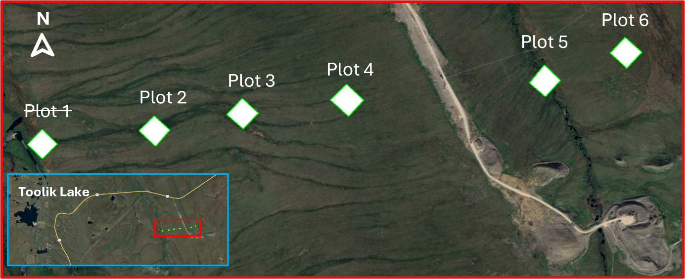
Figure 2. Plot locations. Note that no data from Plot_1 is included in this collection. Inset in the lower left shows broader context in vicinity of Toolik Lake.
Table 7. Plot sampling (0,0) locations, which refers to most southern points that were used for establishing the grid.
| Plot | Latitude | Longitude |
|---|---|---|
| Plot-2 | 68.622031° | -149.362160° |
| Plot-3 | 68.622628° | -149.353266° |
| Plot-4 | 68.623039° | -149.342795° |
| Plot-5 | 68.623666° | -149.323419° |
| Plot-6 | 68.624636° | -149.315580° |
Sampling Protocol
Before sampling at each plot, a 90 m x 90 m grid was formed. These plots consisted of 9 subplots (each 30 m x 30 m) that are aligned with the ABoVE Airborne Campaign coordinate reference system (ESRI:102001 - Canada_Albers_Equal_Area_Conic). Within each subplot another 9 sub-subplots (each 10 m x 10 m) were established. This configuration allowed multi-scale grid-based study of micro heterogeneity at 10 m, 30 m and 90 m scales. The (0, 0) of each plot (most southern point) was determined accurately (within <1 m) using an Emlid GPS device, and each corner of the 90 m x 90 m grid was double checked to stay within <1 m of the desired latitude and longitude coordinates (Table 7).
Grid Labels
As mentioned in Table 1, the ALT labels follow ALT-A-B, where A is the plot numbers (2, 3, 4, 5, and 6), and B is the probing point which goes from 1 to 289 and consists of a 17 x 17 grid cell (5 m each) (Figure 3). Note that not all the points are measured in each plot; further details are provided below. Additionally, the soil samples labels follow Soil-A-B-C-D, where the A is plot number, B shows the subplot number, C shows the sub-subplot number, and finally D shows the number of samples in each core. Figure 3 shows the cores and associated labels of each soil core based on the location in the nested grid. At each plot, the center subplot is labeled as 1 and the remaining subplots from 2 to 9 are labeled clockwise.
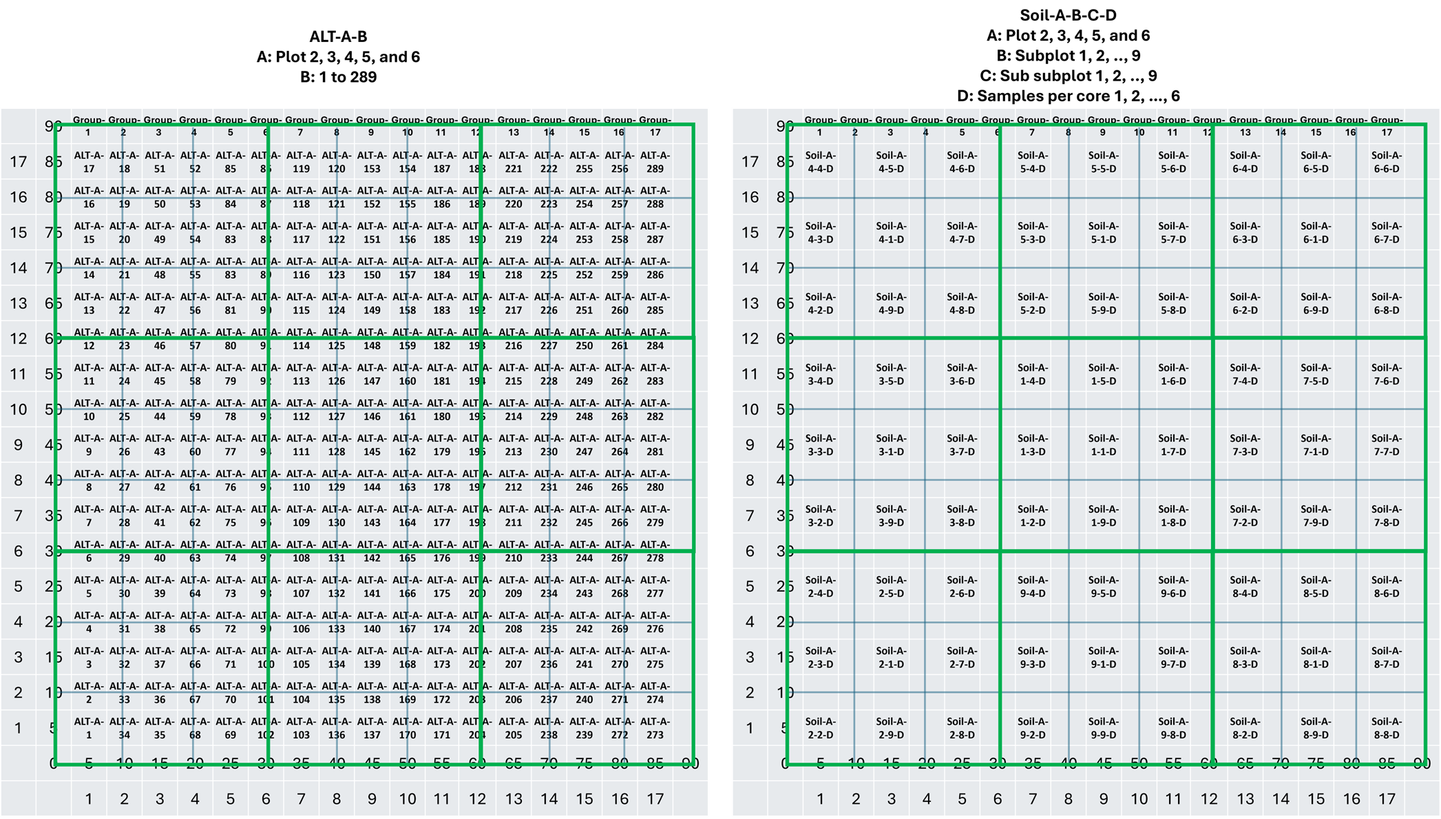
Figure 3. Grid labels. More details of the plot dimensions are provided in Figure 4, the labels in ALT and Soil data are shown in this figure.
Active Layer Thickness
Active layer thickness was measured following the established ABoVE protocol and informed by previous sampling methodologies (Schaefer et al., 2021; ABoVE ALT Protocol). At each location, a metallic rod was inserted into the active layer until refusal, then the rod was taken out of the soil. If the rod hit rock or gravel instead of ice, it was pulled out and re-inserted. Thaw depth measurements do not include the depth of the moss layer. Before pulling the rod out of the soil, a hand is held at the interface of the dead and live moss layers, which is typically exposed by the hole made upon insertion. The thaw depth is the length of the probe to where it is held. This was repeated a minimum of three times for each sampling point, and the mean value was taken as the thaw depth.
It is worth noting that the thickness of the live moss layer was not formally determined. Rather, the thumb (on the upper end of the rod) was inserted until it hit the dead moss layer, which better resists penetration. The rod makes a wide depression in the live moss layer but the dead moss layer resists this, with some very slight compaction, so the thumb stops just above the dead moss layer. That wide depression makes interpretation of where to measure from difficult and, in light of the desire to capture the thickness of the moss layer, it was measured "by feel" with the thumb.
Figure 4 shows the ALT sampling strategy, where the red circles show the location of the ALT sampling. Plot_5 represented the densest sampling, followed by Plot_3 and Plot_4. Plot_6 had abundant rocks and gravel, which considerably slowed measurement and ultimately resulted in only part of that plot being sampled. Plot_2 was sampled more sparsely due to time constraints. The sampling in Plot_5 is conducted with 5-m intervals both in x-y directions, whereas in Plot_3, Plot_4, and Plot_6, it was measured at 10-m intervals in edge subplots (2, 3, …, 9) and 5-m intervals in center subplot 1. These reflect the actual measured points rather than the originally planned sampling grid.
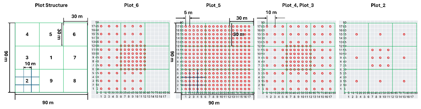
Figure 4. Plot structure and ALT sampling points (red circles). Each original plot is 90 m x 90 m, which consists of 9 subplots (each 30 m x 30 m) shown by green squares. In each subplot there are even smaller (10 m x 10 m) plots, which are denoted in the plot structure by blue squares. Intensive ALT sampling was conducted at 5-m intervals, whereas relaxed sampling was at the 10-m intervals
Soil Sampling
Soil samples were collected at a coarser scale, and ideally in the centers of the 10 m x 10 m plots (a.k.a sub-subplots). The initial focus was to collect soil cores from the top 15 cm soil depth, where 0 includes the top of the green moss layer. In certain plots, two cores were collected back-to-back that cover the top 30 cm of the active layer (Figure 5). Soil sampling was done with a 3 inch x 6 inch AMS soil core sampler (AMS Inc., American Falls, ID). Soil samples were collected in plastic tubes and either processed in the field or preserved to be processed at the Toolik Field Station. Samples from Plot_2 were shipped to the University of Southern California for further processing. More details of the lab measurements are described below in the Lab measurement protocol section. Similar to ALT sampling, Plot_5 contained the most intense sampling, followed by Plot_4, Plot_3, Plot_2, and Plot_6. In Plot_3, and Plot_4. The center plot was sampled deeper to study the 0-30 cm depth (compare blue circles and black circles in Figure 5). At each sampling location, multiple pictures from a handheld digital camera were also taken to characterize the vegetation structure; however, this information is not reported in this dataset. Plot_6 measurements did not go as planned, and after extracting 4 soil cores, the AMS soil core sampler was broken. The site was not revisited due to the presence of substantial rock fragments at the site. Core diameters were 3 inches, and each core was divided into samples that filled a tin container with diameters of 3 inches and a length of ~5 cm, similar to previous sampling procedures (Bakian-Dogaheh et al., 2020; Bakian-Dogaheh et al., 2022).
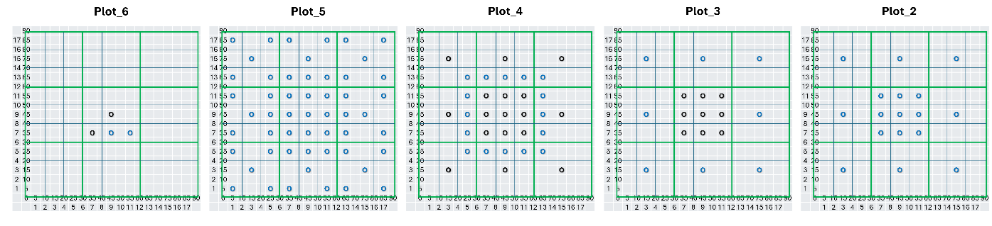
Figure 5. Soil sampling locations, where only top 0-15 cm of the active layer was sampled (blue circles), and locations where two cores were extracted between 0-30 cm (black circles).
Lab Measurement Protocol
Lab samples were either divided and fitted into tin containers in the field or in the lab (Figure 6). Samples in each tin container were measured to record the wet mass and then inserted into an oven and dried at 60 °C for up to 48 hours. During this time, sample weights were measured multiple times to make sure they were dry. The dried mass was then used to calculate bulk density and sample moisture content. The sample volume was equal to the container tin volume, ~251 cm3. Dried samples were then sieved with a 2-mm mesh to extract coarse organic matter, including roots or green/brown moss (dead or live). Additionally, if the sample contained coarse mineral fractions, including rocks and gravels, they were removed in the sieving process and were used to characterize rock fractions.
The dried coarse organic matter was used to characterize the root biomass. The fine earth materials (soil) <2 mm were then shipped to the University of Southern California, and upon proper labeling, the sample was shipped to the Ward Laboratories for soil organic matter measurement using Loss on Ignition (LOI) processing. Additional soil carbon and soil nitrogen measurements were also made using CHN elemental analysis by high temperature combustion techniques. No acidification treatment was used to remove the inorganic carbon in each sample. Therefore, the reported carbon values are the total soil carbon (organic+inorganic). The combustion temperature was around 1350º C, which causes both organic and inorganic carbon to break down. For less organic soils, the mineral texture was also characterized by using the hydrometer method. No organic matter removal was conducted, either via LOI or H2O2 treatment, and the samples contained organic matter during mineral texture analysis. The details of the measurement are similar to those reported in previous studies and datasets, such as Bakian-Dogaheh et al. (2023).
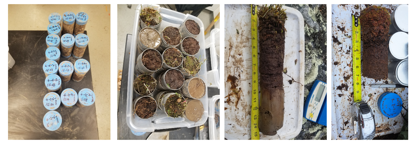
Figure 6. Sample collected in the field. Divided soil cores into tin containers. Soil cores representative of 0-15 and 0-30 (cm) profile.
Soil Roughness Height
Soil roughness height was measured at up to three locations per plot. At each location, a laser range finder was attached to a tape measure on a spirit level at a known height with the support of two tripods (Figure 7). Measurement was conducted with 2-cm intervals for a length of 100 cm in a north-to-south and east-to-west orientation (shown as a cross in Figure 7). Soil roughness height was measured at subplots 1, 4, and 8 in Plot_3, Plot_4, and Plot_5, and only in subplot 1 (center plot) in Plot_2.
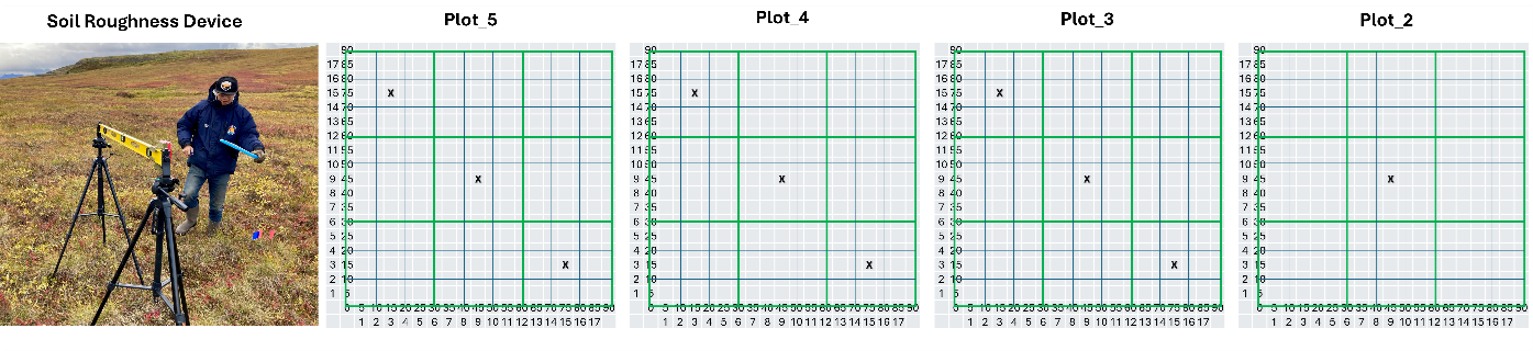
Figure 7. Soil roughness height measurement device and measurement locations within plots.
RGB Optical and Multispectral UAV Survey
UAV imagery was acquired across Plot_2, Plot_3, Plot_4, Plot_5, and Plot_6. UAV flights were conducted between 11:30 am and 3:30 pm on 2024-09-04 using a DJI Matrice 210 v2 at 45 m above ground surface with 80% in-track and sidetrack overlap. RGB imagery was collected at 0.7 cm per pixel using a DJI x7 24mm lens and GPS coordinates were post-processed using KlauPPK Version 7.22.1 to within 3-cm accuracy. Multispectral imagery was collected using the Micasense Red-Edge MX at 3.3 cm per pixel, with the bands as shown in Table 4. Digital Surface Models and Orthomosaics were derived from standard structure-from-motion techniques in Agisoft Metashape Version 2.1.1. NDVI was calculated from multispectral imagery and output as a sixth band. Elevation values fell within 1 m of available Digital Surface Models (NEON, ArcticDEM v4.1). UAV data products were exported to NAD83(2011) UTM 6N coordinate system. The UAV flew at 2.20 m sec-1, and on average, 2.65 pictures sec-1 were collected.
Data Access
These data are available through the Oak Ridge National Laboratory (ORNL) Distributed Active Archive Center (DAAC).
ABoVE: Active Layer Soil Properties and Multispectral Images, Imnavait Creek AK, 2024
Contact for Data Center Access Information:
- E-mail: uso@daac.ornl.gov
- Telephone: +1 (865) 241-3952
References
ABoVE Protocol for ALT Surveys. https://above.nasa.gov/Documents/ALT_Protocol_04.pdf
Bakian-Dogaheh, K., R.H. Chen, Y. Yi, J.S. Kimball, M. Moghaddam, and A. Tabatabaeenejad. 2022. A model to characterize soil moisture and organic matter profiles in the permafrost active layer in support of radar remote sensing in Alaskan Arctic tundra. Environmental Research Letters 17:025011. https://doi.org/10.1088/1748-9326/ac4e37
Bakian-Dogaheh, K., R.H. Chen, M. Moghaddam, Y. Yi, and A. Tabatabaeenejad. 2020. ABoVE: Active Layer Soil Characterization of Permafrost Sites, Northern Alaska, 2018. ORNL DAAC, Oak Ridge, Tennessee, USA. https://doi.org/10.3334/ORNLDAAC/1759
Bakian-Dogaheh, K., R.H. Chen, Y. Yi, T.D. Sullivan, R.J. Michaelides, A.D. Parsekian, K. Schaefer, A. Tabatabaeenejad, J. Kimball, and M. Moghaddam. 2023. Soil Matric Potential, Dielectric, and Physical Properties, Arctic Alaska, 2018. ORNL DAAC, Oak Ridge, Tennessee, USA. https://doi.org/10.3334/ORNLDAAC/2149
Du, J., K.A. Endsley, K. Bakian-Dogaheh, J. Kimball, M. Moghaddam, T. Douglas, A. Melebari, S. Eskandari, J. Kim, J. Whitcomb, Y. Zhao, and S. Henze. 2025. Assessing spatial heterogeneity of active layer thickness over Arctic-foothills tundra through intensive field sampling and multi-source remote sensing. EGUsphere (preprint). https://doi.org/10.5194/egusphere-2025-3236
Schaefer, K., L.K. Clayton, M.J. Battaglia, L.L. Bourgeau-Chavez, R.H. Chen, A.C. Chen, J. Chen, K. Bakian-Dogaheh, T.A. Douglas, S.E. Grelick, G. Iwahana, E. Jafarov, L. Liu, S. Ludwig, R.J. Michaelides, M. Moghaddam, S. Natali, S.K. Panda, A.D. Parsekian, A.V. Rocha, S.R. Schaefer, T.D. Sullivan, A. Tabatabaeenejad, K. Wang, C.J. Wilson, H.A. Zebker, T. Zhang, and Y. Zhao. 2021. ABoVE: Soil Moisture and Active Layer Thickness in Alaska and NWT, Canada, 2008-2020. ORNL DAAC, Oak Ridge, Tennessee, USA. https://doi.org/10.3334/ORNLDAAC/1903