Summary:

The overall purpose in this research was to identify the regions of the world best suited for long-term monitoring of biospheric responses to climate change, i.e. monitoring land surface phenology. Using global 8- km 1982 to 1999 Normalized Difference Vegetation Index (NDVI) data and an eight-element monthly global 1961 to 1990 monthly climatology data, White et al. (2005) identified pixels consistently dominated by annual cycles and then created 500 phenologically and climatically self-similar clusters, which they termed phenoregions. They ranked and screened each phenoregion as a function of landcover homogeneity and consistency, evidence of human impacts, and political diversity. The remaining 140 phenoregions represent areas with a minimized probability of human influence and non-climatic forcings and form elemental units for long-term phenological monitoring (Figure 1). Users should note that the number of screened phenoregions in this data set differ slightly from White et al. (2005). The provided archived phenoregions were screened with a slightly different algorithm.

This data set contains both Binary image and ASCII grid data files and a corresponding .jpg mapfor the 500 elemental phenoregions, for the 140 recommended monitoring phenoregions, and for the 90 ranked clusters. Also included is an ASCII data table containing the descriptive data collected for each of the 500 elemental phenoregions and used for ranking and screening the phenoregions. A users can create their own phenoregion screening criteria using this descriptive information.

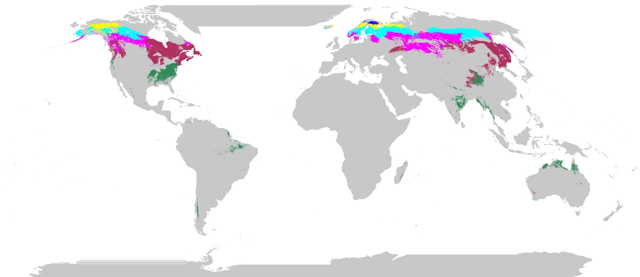
Figure 1. The 140 phenoregions passing the screening factors in Table 1 and best suited for long-term monitoring of climate change.

Data Citation:

Cite this data set as follows:

White M. A., F. M. Hoffman, W. W. Hargrove, and R. R. Nemani. 2005. Phenoregions for Monitoring Vegetation Responses to Climate Change. Data set. Available on-line [http://www.daac.ornl.gov] from Oak Ridge National Laboratory Distributed Active Archive Center, Oak Ridge, Tennessee, U.S.A. doi:10.3334/ORNLDAAC/799.

Table of Contents:

• 1 Data Set Overview
• 2 Data Characteristics
• 3 Applications and Derivation
• 4 Quality Assessment
• 5 Acquisition Materials and Methods
• 6 Data Access
• 7 References

1. Data Set Overview:

Remote sensing of vegetation phenology is an important method with which to monitor terrestrial responses to climate change, but most approaches include signals from multiple forcings, such as mixed phenological signals from multiple biomes, urbanization, political changes, shifts in agricultural practices, and disturbances. Consequently, it is difficult to extract a clear signal from the usually assumed forcing: climate change. Here, using global 8-km 1982 to 1999 Normalized Difference Vegetation Index (NDVI) data and an eight-element monthly climatology, we identified pixels whose wavelet power spectrum was consistently dominated by annual cycles and then created phenologically and climatically self-similar clusters, which we term phenoregions. We then ranked and screened each phenoregion as a function of landcover homogeneity and consistency, evidence of human impacts, and political diversity. Remaining phenoregions represented areas with a minimized probability of non-climatic forcings and form elemental units for long-term phenological monitoring.

The investigators were White, M. A.; Hoffman, F.M.; Hargrove, W.W. and Nemani, R.R.

2. Data Characteristics:

Data File Creation and Description

Elemental Phenoregions

The initial step was to combine the 1982-1999 (not 1994) 10-day composite 8-km Pathfinder Advanced Very High Resolution Radiometer Land (PAL) Normalized Difference Vegetation Index (NDVI) with the eight-element global 1961 to 1990 10 minute monthly climatology data and apply a continuous wavelet transformation to identify pixels with a strong annual cycle which define self-similar climate clusters termed as phenoregions. An iterative k-means clustering approach [Hargrove and Hoffman, 2005] was applied in the development of the 500 elemental phenoregions. Ocean, interrupted space, and land areas not contained in a phenoregion have a value of zero. For all other areas, pixels in each phenoregion contain a unique integer value ranging from 1 to 500. Data are 16-bit signed integers in the global Interrupted Goodes Homolosine projection [DeFries et al., 1998] with projection information as given below. 

Binary Format File:  White_500_elemental_phenoregions.int

Standard ASCII Grid Format File:  White_500_elemental_phenoregions.asc

The companion file, White_500_elemental_phenoregions.jpg, displays these regions and is provided for reference.

Ranked Phenoregions

Second, the 500 elemental phenoregions were ranked and screened to produce 90 cluster rankings. These 90 cluster rankings were determined based on a suite of factors describing their appropriateness to act as climate-response monitoring units. Higher rankings indicate that the given phenoregion is better suited for climate response monitoring. Simply, the abundance of the dominant landcover and consistent information from a vegetation continuous fields product increased rankings whereas cropland, barren, or urban landcovers, evidence of human impacts, and political diversity reduced rankings. Rankings strategies are biome-specific; readers are referred to Table 1 below and White et al. (2005). Data are 16-bit signed integers in the global Interrupted Goodes Homolosine projection [DeFries et al., 1998] with projection information as given below. 

Binary Format File:  White_90_cluster_rankings.int

Standard ASCII Grid Format File:  White_90_cluster_rankings.asc

The companion file, White_90_cluster_rankings.jpg, displays these regions and is provided for reference.

Screened Phenoregions

The 500 elemental phenoregions were combined with the 90 cluster rankings, and the 0 values removed to form 140 final monitoring phenoregions. Data are 16-bit signed integers with projection information as given below.

Binary Format File:  White_140_screened_phenoregions.int

Standard ASCII Grid Format File:  White_140_screened_phenoregions.asc

The companion file, White_140_screened_phenoregions.jpg, displays these ranked clusters and is provided for reference.

Projection Information

Both the binary integer files and the ASCII data files should be projected according to the following information:

Projection_Name=interrupted_goode_homolosine Projection_Code=24 Ellipsoid_Name=sphere Ellipsoid_Code=19 Ellipsoid_Semi-Major_Axis=6370997.000 Ellipsoid_Semi-Minor_Axis=6370997.000 Upper_Left_Corner=-20016000, 8672000 Upper_Right_Corner=20016000, 8672000 Lower_Right_Corner=20016000, -8672000 Lower_Left_Corner=-20016000, -8672000 Geographic_Upper_Left_Corner=180d00'00.0000W,090d00'00.0000N; Geographic_Upper_Right_Corner=180d00'00.0000E,090d00'00.0000N; Geographic_Lower_Right_Corner=180d00'00.0000E,090d00'00.0000S; Geographic_Lower_Left_Corner=180d00'00.0000W,090d00'00.0000S; Number_Of_Lines=2168 Pixels_Per_Line=5004 Pixel_Resolution=8000,8000 Pixel_Resolution_Units=meters

Descriptive data collected for each of the 500 elemental phenoregions and used for ranking and screening the phenoregions.

White_ancillary_phenoregion_data.txt.

Users may desire to create their own screening/selection criteria with the descriptive information provided for each of the 500 elemental phenoregions. This tabular data may then be cross-referenced to the 500 elemental phenoregions to develop unique criteria. Each line contains information for one of the clusters in White_500_elemental_phenoregions.int.

Column Content Name	Units	Description
Column cluster	dimensionless	Can be used to cross reference cluster numbers in figure 1.
Column npixels	dimensionless	The number of pixels.
Column dom_lc	categorical	The dominant categorical landcover. 1=evergreen needleleaf forest; 2=evergreen broadleaf forest; 3=deciduous needleleaf forest; 4=deciduous broadleaf forest; 5=mixed forest; 6=woodland; 7=wooded grassland; 8=closed shrubland; 9=open shrubland; 10=grassland; 11=crop; 12=barren; 13=urban.
Column %dom_lc	percent	The cover by the dominant categorical landcover.
Column neglc	percent	The cover by crop + urban + barren categorical landcovers.
Column tree	percent	The mean tree cover from the vegetation continuous fields product [Hansen et al., 2003]. Note that for 34 clusters, nearest neighbor resampling did not produce land values from the vegetation continuous fields data. This occurred only in very sparse clusters (less than seven pixels) and had no impact on selection of the monitoring phenoregions. Also applies to herb and bare columns. For these situations, a fill value of -999 is used.
Column herb	percent	The mean herbaceous cover from the vegetation continuous fields product [Hansen et al., 2003].
Column bare	percent	The mean bare cover from the vegetation continuous fields product [Hansen et al., 2003].
Column hfoot	dimensionless	The mean human footprint [Sanderson et al., 2002]. Evidence of human impacts ranges from 0 (lowest) to 100 (highest).
Column poldiv	dimensionless	The political diversity based on a Simpson's diversity index [Simpson, 1949] and gridded country information [CIESIN, 2000]. Ranges from 0 (phenoregion occupied by only one country) to 100 (infinite diversity).
Column prec	mm	The annual average total precipitation [New et al., 2002].
Column tavg	deg C	The annual average temperature [New et al., 2002].

Example Data Records

cluster npixels dom_lc %dom_lc neglc tree herb bare hfoot poldiv prec tavg 1 3646 13 65 65 25 70 5 1 1 720 -5.4 2 2073 1 76 11 26 60 15 12 0 448 5.0 3 2465 1 46 4 43 56 1 29 56 1189 9.3 4 1 13 100 100 -999 -999 -999 7 0 408 -6.9 5 5771 10 82 9 0 24 76 12 62 213 6.8 ... 495 4895 10 34 30 13 69 19 12 63 409 -4.9 496 152 1 47 1 44 56 0 11 18 1588 5.5 497 1 13 100 100 -999 -999 -999 5 0 516 -8.7 498 315 13 72 98 3 19 81 4 18 388 -8.6 499 3940 3 71 0 47 51 2 4 0 402 -7.8 500 1344 4 49 16 19 79 2 4 6 648 -2.4

The header line can be read as 12A8; the data lines are 11I8,F8.1.

Site boundaries: (All latitude and longitude given in degrees and fractions)

Site (Region)	Westernmost Longitude	Easternmost Longitude	Northernmost Latitude	Southernmost Latitude	Geodetic Datum
Global (gridded)	-180	180	90	-90

Time period:

The data set covers the period 1982/01/01 to 1999/12/31. (1994 not used because of sensor failure)

3. Data Application and Derivation:

Vegetation phenology, the study of the timing of recurring vegetation cycles such as canopy emergence and senescence, is an emerging field of climate change science. Yet many ground-based and modeling studies are biased towards biomes (deciduous broadleaf forest) and regions (western Europe) that, from a global perspective, are nearly irrelevant. Additionally, in remote sensing studies focusing on global patterns, observed trends are subject to multiple and often unknown non-climatic forcings and technical problems.

In spite of these difficulties, there is a clear need for continued phenological monitoring. Observational modeling and remote sensing evidence suggests that vegetation phenology is changing in response to warming climates, principally through an earlier start of season (SOS) and later end of season (EOS). Through these types of studies, vegetation phenology can be used as a sensitive barometer of terrestrial responses to short- and long-term climate variability.

Climate change usually is assumed to be the primary forcing of trends or turning points in SOS and/or EOS timeseries; while this may be true in many cases, especially when analyzed over large regions, a variety of factors may influence observed trends. Nonclimatic forcings of observed shifts in vegetation phenology include urbanization, the collapse of political systems, and disturbances. Further, while independent lines of evidence tend to show similar overall trends, geographically coincident data are often weakly correlated, complicating attempts to extract a clear vegetative signal from potentially confounding factors (variation in soil wetness, trends in snow cover, degradation of remote sensing platforms, variable within-pixel phenological trends).

In response to the need for a monitoring strategy that targets climate change impacts and provides geographical units for trend attribution and fine resolution remote sensing studies, we propose the use of a limited number of phenologically and climatically self-similar clusters. There are four central features of our proposed strategy: (1) identification of pixels with a strong annual cycle; (2) creation of clusters with similar vegetation phenology and climate; (3) removal of clusters dominated by human-related landcover; (4) selection of remaining clusters with homogeneous landcover, low evidence of human impacts, and low diversity of political units. This approach, which identifies clusters of pixels with an easily identifiable seasonal signal, is designed to maximize the potential for detecting climate forcings while minimizing the influence of landcover, human, and political influences. As such, these identified phenoregions can form the basis for a global phenological monitoring network.

4. Quality Assessment:

We obtained the 1982-1999 (1994 not used because of sensor failure) 10-day composite 8-km Pathfinder Advanced Very High Resolution Radiometer Land (PAL) Normalized Difference Vegetation Index (NDVI) data set. The PAL data set contains extensive artifacts related to within- and among-sensor calibration, volcanic eruptions, and water vapor. By intentionally selecting the PAL dataset, we implemented an extremely conservative approach: only those pixels whose annual cycle is stronger than the inherent PAL noise passed our initial filter.

Our approach, which was designed only to select optimal regions, not to represent the possible distribution of biome/climate combinations, strongly suggests that a limited region of the globe is suitable for climate response monitoring with coarse resolution sensors. Other regions, especially those dominated by precipitation variability, are also likely to be highly responsive to climate change and are not included here. For these critical regions in which coarse resolution monitoring is not optimal or in which other factors are likely to confound results, we advocate the use of finer resolution sensors and ground observations coupled with landcover and landuse histories, and the comparison of protected and non-protected regions.

5. Data Acquisition Materials and Methods:

We obtained the 1982-1999 (1994 not used because of sensor failure) 10-day composite 8-km Pathfinder Advanced Very High Resolution Radiometer Land (PAL) Normalized Difference Vegetation Index (NDVI) dataset. Next, we conducted a continuous wavelet transformation of the 612-element NDVI timeseries for each pixel. We calculated annual time averaged local wavelet spectra and identified pixels in which the annual time scale was dominant in at least 15 of 17 possible years. This step identified the 1,012,866 pixels for which the annual scale was consistently strong and therefore tractable for coarse resolution phenology monitoring. Nearly all arid shrublands, deserts, and moist tropical forests were eliminated.

We then used an iterative k-means clustering approach [Hargrove and Hoffman, 2005] of the PAL NDVI and an eight-element global 1961 to 1990 monthly climatology that included precipitation, wet-day frequency, temperature, diurnal temperature range, relative humidity, sunshine duration, ground frost frequency and windspeed [New et al., 2002] reprojected to the 8 km PAL Goodes Interrupted Homolosine projection to identify the groups of pixels forming the elemental monitoring units. The clustering approach, performed on an Oak Ridge National Laboratory parallel supercomputer, generated n initial cluster centroids spaced evenly in the 708-axis hyperspace (all data were normalized to a mean of zero and a unit variance, individually by axis). Each pixel was then assigned to the centroid with the nearest Euclidian distance. Mean centroid locations were recalculated based on the assigned pixels and the process was repeated until less than 0.05% of pixels were reassigned. Although techniques exist to reduce the dimensionality of clustering inputs, the inclusion of correlated axes does not strongly affect final grouping. Given that sets of axes without perfect correlation (as will occur with landcover changes or disturbances) can add discriminatory information and that axes used here represent either a climate descriptor or NDVI at a particular date, we chose to retain all axes.

We experimented with a range of clusters from 10 to 1000 and found that 500 clusters provided an optimal separation such that clusters tended to exist on only one continent and the distribution did not contain a high frequency of minimally represented clusters. We created three clusterings: (1) climate alone, (2) NDVI alone; and (3) climate and NDVI. Climate alone produced large homogeneous clusters; NDVI alone produced large numbers of clusters with only one or a few pixels; NDVI and climate provided good representation of distinctions in landcover and topography without creation of numerous sparse clusters. We adopted use of the NDVI and climate clusters, which we term phenoregions. The phenoregions capture well known vegetation features, such as precipitation gradients in Sahelian Africa, the mesic periphery of Australia, and extensive crop-dominated regions of the Midwestern United States. Use of the PAL data will tend to create phenoregions with similar satellite contamination, a useful characteristic for assessing long-term trend attribution between corrected and uncorrected NDVI datasets.

Selection of Clusters: At this stage, the 500 climatically and phenologically self-similar phenoregions represented groups of pixels appropriate for the formation of spatially composited timeseries. We then used a four-step process to identify phenoregions, by landcover, with characteristics likely to maximize their utility for climate-response monitoring.

First, to minimize the incidence of sparse clusters and consequent potential for georegistration/georectification difficulties, we removed all clusters with fewer than 100 pixels. Second, we removed clusters if the categorical landcover [DeFries et al., 1998] with the highest percent cover was crop, barren, or urban, all of which are likely to be responsive to non-climatic forcings. Third, we implemented a ranking system designed to represent quantitatively the suitability of the remaining 211 clusters for climate response monitoring. Simply, the abundance of the dominant landcover and consistent information from a vegetation continuous fields product increased rankings whereas cropland, barren, or urban landcovers, evidence of human impacts, and political diversity reduced rankings. See Table 1 for details. Fourth, we used elements of the same ranking system in a filter to eliminate clusters with low scores in one or more categories.

The remaining 140 phenoregions existed almost exclusively in mid to high latitudes of North America and Eurasia. In this final selection, the dominant biomes were evergreen needleleaf forest and woodlands. Grasslands, mixed forests, and deciduous needleleaf forests were well represented whereas evergreen broadleaf forests, deciduous broadleaf forests, and wooded grasslands were sparse. The selected evergreen broadleaf forest phenoregions existed in seasonally dry regions; no equatorial moist tropical forest was selected. No arid shrublands were selected. Given that much of the NDVI amplitude in northern forests is related to annual snow cover patterns, monitoring in these abundant phenoregions should focus on trend attribution to snow versus vegetation dynamics. This decoupling of low canopy amplitude in many boreal forests from a strong snowmelt signal is challenging with AVHRR records and should be a focus of future ground campaigns linked to multi-resolution remote sensing.

With the exception of a phenoregion in southeastern Madagascar (barely visible at top), Africa was removed, usually as a result of high political diversity within the longitudinally extensive phenoregions. Small dry evergreen broadleaf forest phenoregions existed in South America but the continent, in general, did not pass our screening criteria. The single wooded grassland phenoregion spanned nearly the entirety of northern Australia. The deciduous broadleaf forest and western European regions were minimally represented.

Table 1. Ranking and Screening of Phenoregions^a

Variable	Ranking Impact	Cluster Acceptable If
pixels	NA	>100
dominant landcoverb	NA	Not crop, urban, or barren
percent dominant landcoverb	+	>30%
percent urban + crop + barrenb	-	<30%
mean percent bare coverc	-	<30%
mean percent tree coverc	+ for forests	forests >30%
		10% > woodland < 60%
		10% > wooded grassland < 40%
mean percent herbaceous coverc	+ for grassland	grasslands >40%
		woodlands >20%
		wooded grasslands >40%
mean human footprintd	-	<30
political diversitye	-	<50
aFor ranking, variables were calculated or averaged for the phenoregion and added (+) or subtracted (−). Note that for woodlands and wooded grasslands, the vegetation continuous fields were not used. All rankings were scaled from 0 to 100. Clusters were accepted as a valid phenoregions if the listed conditions were met. Acceptability criteria are not absolute; users are encouraged to develop customized screenings using the archived supporting materials. All data existed or were reprojected to the 8 km global Goode's Homolosine projection. See White et al. (2005) for more details. bCategorical landcover [DeFries et al., 1998] with the highest percent cover. cFrom vegetation continuous fields product [Hansen et al., 2003]. dBased on population, land transformation, accessibility, and stable electrical light sources [Sanderson et al., 2002]. Dimensionless from 0 (no human footprint) to 100 (highest possible human footprint). eBased on Center for International Earth Science Information Network (Gridded population of the world (GPW), version 2, 2000, available at http://sedac.ciesin.columbia.edu/plue/gpw) and Simpson's diversity index [Simpson, 1949]. Ranges from 0 (phenoregion contains only one country) to 100 (infinite number of countries).

6. Data Access:

This data is available through the Oak Ridge National Laboratory (ORNL) Distributed Active Archive Center (DAAC) or the EOS Data Gateway.

Data Archive Center:

Contact for Data Center Access Information:

E-mail: uso@daac.ornl.gov
Telephone: +1 (865) 241-3952
FAX: +1 (865) 574-4665

Product Availability:

...Requested data can be provided electronically on the ORNL DAAC's anonymous FTP site or on various media including, CD-ROMs, 8-MM tapes, or diskettes.

Reading the Media:

(To be completed manually by Document Curator)

Software and Analyses Tools:

(To be completed manually by Document Curator)

7. References:

CIESIN, Gridded Population of the World (GPW), Version 2, Center for International Earth Science Information Network (Columbia University); International Food Policy Research Institute; and World Resources Institute, Palisades (NY), 2000.

DeFries, R., M. Hansen, J.R.G. Townshend, and R. Sohlberg, Global land cover classifications at 8 km spatial resolution: The use of training data derived from Landsat imagery in decision tree classifiers, International Journal of Remote Sensing, 19, 3141-3168, 1998.

Hansen, M.C., R. DeFries, J. Townshend, M. Carroll, C. Dimiceli, and R. Sohlberg, Global percent tree cover at a spatial resolution of 500 meters: first results of the MODIS vegetation continuous fields algorithm, Earth Interactions, 7, Paper No. 10, 2003.

Hargrove, W. W., and F. M. Hoffman (2005), The potential of multivariate quantitative methods for delineation and visualization of ecoregions, Environ. Manage., in press.

New, M., D. Lister, M. Hulme, and I. Makin, A high-resolution data set of surface climate over global land areas, Climate Research, 21, 1-25, 2002.

Sanderson, E., J. Malanding, M. Levy, K. Redford, A. Wannebo, and G. Woolmer, The human footprint and the last of the wild, BioScience, 52, 891-904, 2002. Simpson, E.H., Measurement of diversity, Nature, 163, 688, 1949.

Simpson, E.H., Measurement of diversity, Nature, 163, 688, 1949.

White M. A., F. Hoffman, W. W. Hargrove, R. R. Nemani. 2005. A global framework for monitoring phenological responses to climate change, Geophys. Res. Lett., 32, L04705, doi:10.1029/2004GL021961.

8. Document Information: