Documentation Revision Date: 2018-04-02
Data Set Version: 1
Summary
This dataset provides Landsat phenology algorithm (LPA) derived start and end of growing seasons (SOS and EOS) at 500-m resolution for deciduous and mixed forest areas of 75 selected Landsat sidelap regions across the Eastern United States and Canada. The data are a 30-year time series (1984-2013) of derived spring and autumn phenology for forested areas of the Eastern Temperate Forest, Northern Forest, and Taiga ecoregions.
The study used Landsat TM/ETM+ images acquired between 1984 and 2013 for 75 Landsat sidelap regions. Sidelaps were selected using a stratified random sampling approach within three United States Environmental Protection Agency Level I ecoregions: Northern Forest, Taiga, and Eastern Temperate Forest. The Landsat phenology algorithm (LPA) (Melaas et. al, 2013, 2016) was used to estimate the day of year (DOY) associated with leaf emergence at the start of the growing season (SOS) and autumn senescence at the end of growing seasons (EOS) for deciduous and mixed forest 30-m Landsat pixels. Data were aggregated to 500-m spatial resolution using the MODIS grid.
Additional data include the number of years of detected mean Landsat-detected spring onset and autumn onset dates, subsequent trend magnitude (Theil-Sen) and significance (Mann-Kendall) values, as well as location information including Landsat tile numbers, MODIS pixel coordinates, and ecoregion.
This dataset includes 75 files with phenology data in comma-separated (.csv) format and one shapefile (.shp) with the ecoregions locations. The shapefile is also provided in *.kmz format for viewing in Google Earth.
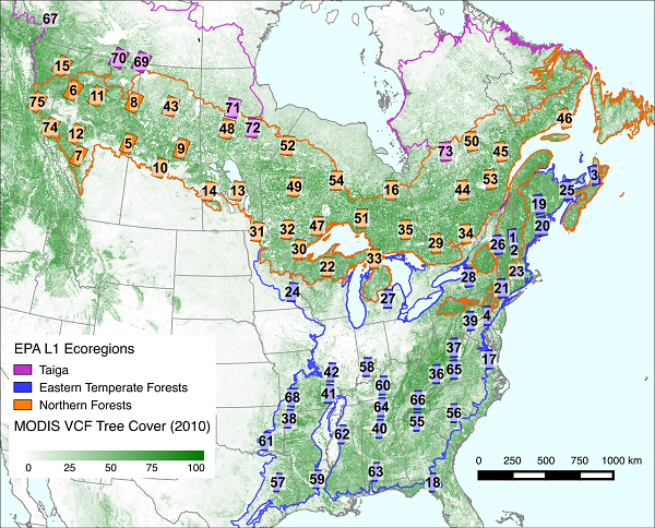
Figure 1. Map of the 75 selected Landsat sidelap regions within the three United States Environmental Protection Agency Level I ecoregions. From Melaas et al., 2018.
Citation
Melaas, E.K., M.A. Friedl, and D. Sulla-Menashe. 2018. Landsat-derived Spring and Autumn Phenology, Eastern US - Canadian Forests, 1984-2013. ORNL DAAC, Oak Ridge, Tennessee, USA. https://doi.org/10.3334/ORNLDAAC/1570
Table of Contents
- Data Set Overview
- Data Characteristics
- Application and Derivation
- Quality Assessment
- Data Acquisition, Materials, and Methods
- Data Access
- References
Data Set Overview
The study used Landsat TM/ETM+ images acquired between 1984 and 2013 for 75 Landsat sidelap regions. Sidelaps were selected using a stratified random sampling approach within three United States Environmental Protection Agency Level I ecoregions: Northern Forest, Taiga, and Eastern Temperate Forest. The Landsat phenology algorithm (LPA) (Melaas et. al, 2013, 2016) was used to estimate the day of year (DOY) associated with leaf emergence at the start of the growing season (SOS) and autumn senescence at the end of growing seasons (EOS) for deciduous and mixed forest 30-m Landsat pixels. Data were aggregated to 500-m spatial resolution using the MODIS grid.
Additional data include the number of years of detected mean Landsat-detected spring onset and autumn onset dates, subsequent trend magnitude (Theil-Sen) and significance (Mann-Kendall) values, as well as location information including Landsat tile numbers, MODIS pixel coordinates, and ecoregion.
What is a sidelap? For Landsat satellites to provide nearly complete coverage of the Earth’s surface with 185-km wide image swaths (later Landsats have wider swaths), some overlapping of orbits was required. The amount of swath overlap or sidelap varies from 7-14 percent at the Equator to a maximum of approximately 85 percent at 81 degrees north or south latitude. In these areas where overlap or sidelap occurred, more images are available, and this increases the likelihood that more good quality images (i.e., no clouds) will be available for analyses.
Related Publication
Melaas, E. K., M. A. Fridel, and D. Sulla-Menashe. 2018. Multidecadal Changes and Interannual Variation in Springtime Phenology of North American Temperate and Boreal Deciduous Forests. Geophysical Research Letters. https://doi.org/10.1002/2017GL076933
Related Datasets
Elmore, A.J., D. Nelson, S.M. Guinn, and R. Paulman. 2017. Landsat-based Phenology and Tree Ring Characterization, Eastern US Forests, 1984-2013. ORNL DAAC, Oak Ridge, Tennessee, USA. http://dx.doi.org/10.3334/ORNLDAAC/1369
Data Characteristics
Spatial Coverage: Eastern United States and Canada
Spatial Resolution: 500-m
Temporal Coverage: 1984-01-01 to 2013-12-31
Temporal Resolution: Annual
Study Areas (All latitude and longitude given in decimal degrees)
| Site | Westernmost Longitude | Easternmost Longitude | Northernmost Latitude | Southernmost Latitude |
|---|---|---|---|---|
| Eastern US and Canada | -124.424 | -60.3954 | 62.0367 | 29.6345 |
Data File Information
SOS and EOS Timeseries Data
There are 75 files in comma-separated format (.csv), one for each of the selected sidelap regions across the Eastern United States and Canada
Each file provides the following data for a specific slidelap region:
- Each row represents a 500-m MODIS pixel with identified deciduous and mixed forest 30-m Landsat pixels. Thus, each row in a file corresponds to a potential 30-year timeseries of mean SOS and EOS as DOY for the MODIS pixel.
- But, many MODIS pixels have no (zero) Landsat pixels where SOS and EOS could be detected and all spring and autumn DOY columns are “NA”.
- For MODIS pixels with Landsat pixels where SOS and EOS could be derived for some years, those yearly spring and autumn values are the mean SOS and EOS as Julian days of those forest 30-m Landsat pixels as aggregated to a 500-m MODIS pixel for that year, potentially years 1984 through 2013.
- Together then, all the rows in a file are all the MODIS pixels in the sidelap region with identified deciduous and mixed forest Landsat pixels.
- Coordinates (centroids) and MODIS grid identifiers are provided for each MODIS pixel.
- For MODIS pixels with Landsat pixels where SOS and EOS could be derived, the total number of years of available data for spring and for autumn in the row are provided.
- Trend analysis magnitude (Theil-Sen) and significance (Mann-Kendall) values are included for SOS and EOS timeseries.
File naming conventions
The files are named as phenology_sceneX_site_YYY_name.csv
Where:
_sceneX is the sidelap number
_site_YYY is the Level 2 Ecoregion, and
_name refers to a location for reference purposes (forest name, town, or other location) in the sidelap.
Refer to Table 2 for the ecoregions and Table 3 for locations of the sidelaps.
Example file name:
phenology_scene23_site_mwp_harvard.csv
This file provides data for scene 23, a mixed wood plains Level 2 Ecoregion in the Harvard Forest.
Data Dictionary
Any missing data denotes that either SOS or EOS phenology dates were undetectable due to missing or poor quality Landsat imagery during the greenup and greendown periods when phenology dates are typically detected. Missing data are indicated with NA.
Table 1. Variables in the .csv data files
| Column name | Units | Description |
|---|---|---|
| latitude | Decimal degrees | Latitude of the 500-m MODIS pixel centroid |
| longitude | Decimal degrees | Longitude of the 500-m MODIS pixel centroid |
| tile_h | Corresponding horizontal MODIS tile of 500-m pixel | |
| tile_v | Corresponding vertical MODIS tile of 500-m pixel | |
| line | Line number of MODIS pixel | |
| samp | Sample number of MODIS pixel | |
| tile | Corresponding MODIS tile name | |
| num_pix | count | Number of deciduous and mixed forest 30-m Landsat pixels located within the 500-m MODIS pixel |
| num_spr | count | Number of years of LPA detected SOS |
| num_aut | count | Number of years of LPA detected EOS |
| spr_1984 to spr_2013 (30 columns) | DOY | Detected SOS date (Julian day of year). Value is mean SOS of forest 30-m Landsat pixels as aggregated to a 500-m MODIS pixel for that year, potentially 1984 through 2013. |
| aut_1984 to aut_2013 (30 columns) | DOY | Detected EOS date (Julian day of year). Value is mean EOS of forest 30-m Landsat pixels as aggregated to a 500-m MODIS pixel for that year, potentially 1984 through 2013. |
| ts_spr | Theil-Sen trend magnitude estimate for spring phenology time series | |
| mk_spr | Mann-Kendall trend significance for spring phenology time series; | |
| ts_aut | Theil-Sen trend magnitude estimate for autumn phenology time series | |
| mk_aut | Mann-Kendall trend significance for autumn phenology time series |
Table 2. EPA Level 1 and Level 2 Ecoregions in the 75 sidelaps
| Level 1 Ecoregion Code | Level 1 Ecoregion | Level 2 Ecoregion Code | Level 2 Ecoregion |
|---|---|---|---|
| ETF | Eastern Temperate Forest | AH | Atlantic Highlands |
| ETF | Eastern Temperate Forest | MA | Mid Atlantic Coastal Plain |
| ETF | Eastern Temperate Forest | MWP | Mixed Wood Plains |
| ETF | Eastern Temperate Forest | OA | Ozark/Ouachita Appalachian Forest |
| ETF | Eastern Temperate Forest | SUP | Southeastern USA Plains |
| ETF | Eastern Temperate Forest | TEP | Temperate Prairies |
| NF | Northern Forest | BP | Boreal Plain |
| NF | Northern Forest | HP | Hudson Plain |
| NF | Northern Forest | MWP | Mixed Wood Plains |
| NF | Northern Forest | MWS | Mixed Wood Shield |
| NF | Northern Forest | TS | Taiga Shield |
| NF | Northern Forest | WC | Western Cordillera |
| T | Taiga | TC | Taiga Cordillera |
| T | Taiga | TP | Taiga Plain |
| T | Taiga | TS | Taiga Shield |
Table 3. Characteristics of sidelap scenes. The scene locations are intended to serve as a general reference to the country and state or province and the ecoregions. Included for each scene is the "site_YYY_name" used in the respective data file name.
| Scene # | Scene Reference Location | State or Province, Country | Level 1 Ecoregion | Level 2 Ecoregion | site_YYY_name |
|---|---|---|---|---|---|
| 1 | Bartlett | New Hampshire, USA | ETF | AH | ah_bartlett |
| 2 | Hubbard | New Hampshire, USA | ETF | AH | ah_hubbard |
| 3 | Nova Scotia | Nova Scotia, CA | ETF | AH | ah_nova_scotia |
| 4 | Philadelphia | Pennsylvania, USA | ETF | AH | ah_philadelphia |
| 5 | Bonnyville | Alberta, CA | NF | BP | bp_bonnyville |
| 6 | Chinchaga | Alberta, CA | NF | BP | bp_chinchaga |
| 7 | Edmonton | Alberta, CA | NF | BP | bp_edmonton |
| 8 | Fort Mcmurray | Alberta, CA | NF | BP | bp_fort_mcmurray |
| 9 | La Ronge | Saskatchewan, CA | NF | BP | bp_la_ronge |
| 10 | Saskatoon | Saskatchewan, CA | NF | BP | bp_saskatoon |
| 11 | Wabasca | Alberta, CA | NF | BP | bp_wabasca |
| 12 | Whitecourt | Alberta, CA | NF | BP | bp_whitecourt |
| 13 | Winnipeg | Manitoba, CA | NF | BP | bp_winnipeg |
| 14 | Yorkton | Manitoba, CA | NF | BP | bp_yorkton |
| 15 | Zama | British Columbia, CA | NF | BP | bp_zama |
| 16 | Kesagami | Ontario, CA | NF | HP | hp_kesagami |
| 17 | Chesapeake | Virginia, USA | ETF | MA | ma_chesapeake |
| 18 | Tallahassee | Florida, USA | ETF | MA | ma_tallahassee |
| 19 | Acadia | New Brunswick, CA | ETF | MWP | mwp_acadia |
| 20 | Bar Harbor | Maine, USA | ETF | MWP | mwp_bar_harbor |
| 21 | Cary | New York, USA | ETF | MWP | mwp_cary |
| 22 | Green Bay | Wisconsin, USA | NF | MWP | mwp_green_bay |
| 23 | Harvard | Massachusetts, USA | ETF | MWP | mwp_harvard |
| 24 | Minneapolis | Minnesota, USA | ETF | MWP | mwp_minneapolis |
| 25 | Moncton | New Brunswick, CA | ETF | MWP | mwp_moncton |
| 26 | Proctor | Vermont, USA | ETF | MWP | mwp_proctor |
| 27 | Saginaw | Michigan, USA | ETF | MWP | mwp_saginaw |
| 28 | Syracuse | New York, USA | ETF | MWP | mwp_syracuse |
| 29 | Algonquin | Ontario, CA | NF | MWS | mws_algonquin |
| 30 | Boundary Waters | Minnesota, USA | NF | MWS | mws_boundary_waters |
| 31 | Grand Forks | Minnesota, USA | NF | MWS | mws_grand_forks |
| 32 | Kabetogama | Ontario, CA | NF | MWS | mws_kabetogama |
| 33 | Mackinac | Michigan, USA | NF | MWS | mws_mackinac |
| 34 | Ottawa | Ontario, CA | NF | MWS | mws_ottawa |
| 35 | Sudbury | Ontario, CA | NF | MWS | mws_sudbury |
| 36 | Charleston | West Virginia, USA | ETF | OA | oa_charleston |
| 37 | Dolly Sods | West Virginia, USA | ETF | OA | oa_dolly_sods |
| 38 | Fayetteville | Arkansas, USA | ETF | OA | oa_fayetteville |
| 39 | Harrisburg | Pennsylvania, USA | ETF | OA | oa_harrisburg |
| 40 | Huntsville | Alabama, USA | ETF | OA | oa_huntsville |
| 41 | Mark Twain | Missouri, USA | ETF | OA | oa_mark_twain |
| 42 | St Louis | Illinois, USA | ETF | OA | oa_st_louis |
| 43 | Cree | Saskatchewan, CA | NF | SS | ss_cree |
| 44 | Gouin | Quebec, CA | NF | SS | ss_gouin |
| 45 | Manicouagan | Quebec, CA | NF | SS | ss_manicouagan |
| 46 | Mingan | Quebec, CA | NF | SS | ss_mingan |
| 47 | Nipigon | Ontario, CA | NF | SS | ss_nipigon |
| 48 | Nobs | Manitoba, CA | NF | SS | ss_nobs |
| 49 | Pipestone | Ontario, CA | NF | SS | ss_pipestone |
| 50 | Pletipi | Quebec, CA | NF | SS | ss_pletipi |
| 51 | Pukaskwa | Ontario, CA | NF | SS | ss_pukaskwa |
| 52 | Sachigo | Ontario, CA | NF | SS | ss_sachigo |
| 53 | Saguenay | Quebec, CA | NF | SS | ss_saguenay |
| 54 | Winisk | Ontario, CA | NF | SS | ss_winisk |
| 55 | Atlanta | Georgia, USA | ETF | SUP | sup_atlanta |
| 56 | Charlotte | South Carolina, USA | ETF | SUP | sup_charlotte |
| 57 | Davy Crockett | Texas, USA | ETF | SUP | sup_davy_crockett |
| 58 | Indianapolis | Indiana, USA | ETF | SUP | sup_indianapolis |
| 59 | Kisatchie | Louisiana, USA | ETF | SUP | sup_kisatchie |
| 60 | Mammoth Cave | Kentucky, USA | ETF | SUP | sup_mammoth_cave |
| 61 | Mcalester | Oklahoma, USA | ETF | SUP | sup_mcalester |
| 62 | Memphis | Mississippi, USA | ETF | SUP | sup_memphis |
| 63 | Montgomery | Alabama, USA | ETF | SUP | sup_montgomery |
| 64 | Nashville | Tennessee, USA | ETF | SUP | sup_nashville |
| 65 | Roanoke | Virginia, USA | ETF | SUP | sup_roanoke |
| 66 | Smoky Purchase | Tennessee, USA | ETF | SUP | sup_smoky_purchase |
| 67 | Nahanni | Northwest Territories, CA | T | TC | tc_nahanni |
| 68 | Springfield | Missouri, USA | ETF | TEP | tep_springfield |
| 69 | Athabasca | Northwest Territories, CA | T | TP | tp_athabasca |
| 70 | Slave | Northwest Territories, CA | T | TP | tp_slave |
| 71 | Amisk | Manitoba, CA | T | TS | ts_amisk |
| 72 | Gillam | Manitoba, CA | T | TS | ts_gillam |
| 73 | Mistassini | Quebec, CA | T | TS | ts_mistassini |
| 74 | Wc Kakwa | Alberta, CA | NF | WC | wc_kakwa |
| 75 | Wc Williston | British Columbia, CA | NF | WC | wc_williston |
Shapefile with sidelap locations
The shapefile is provided in the compressed file Phenology_Landsat_Sidelap_Regions_US_CA.zip. The data are also provided as a companion file in .kmz format for viewing in Google Earth.
The shapefile provides the 75 sidelaps (scenes), as polygons. Bounding boxes for the scenes can be extracted from the scene polygons in the Shapefile.
Table 4. Attributes in the shapefile Phenology_Landsat_Sidelap_Regions_US_CA
| Attribute | Description |
|---|---|
| FID | Number of sites (1-75) |
| Scene: X_location | Corresponds to locations in the broader ecoregions. The X corresponds to the abbreviation for the level 2 ecoregion of the location. Refer to Table 3. Example: ah_bartlett |
| L1 | Level 1 ecoregion associated with each scene (sidelap). Refer to Table 3. |
Application and Derivation
Results from this work support the utility of land surface phenology information derived from Landsat for improving information and understanding of ecosystem processes at landscape scales.
Quality Assessment
The assessment and validation of remotely sensed estimates of SOS and EOS dates with the Landsat phenology algorithm (LPA) was reported in Melaas et al. (2016).
Data Acquisition, Materials, and Methods
Overview
The Landsat phenology algorithm (LPA) described by Melaas et al. (2013) and subsequently refined and validated in Melaas et al. (2016) was used to estimate the long-term average and the annual day of year (DOY) associated with leaf emergence (start of growing season: SOS) and autumn senescence (end of growing season: EOS) at 30-m spatial resolution from time series of Landsat 4, 5, and 7 images. This study used the LPA to focus on retrieval and analysis of SOS and EOS detection for forest pixels (Melaas et al., 2018).
What is a sidelap? For Landsat satellites to provide nearly complete coverage of the Earth’s surface with 185-km wide image swaths (later Landsats have wider swaths), some overlapping of orbits was required. The amount of swath overlap or sidelap varies from 7-14 percent at the Equator to a maximum of approximately 85 percent at 81 degrees north or south latitude. In these areas where overlap or sidelap occurred, more images are available, and this increases the likelihood that more good quality images (i.e., no clouds) will be available for analyses.
Site Selection
Data used were Landsat TM/ETM+ imagery acquired between 1984 and 2013 for 75 Landsat sidelaps located in the Eastern United States and Canada. Landsat sidelaps were selected using a stratified random sampling of sidelaps located within the United States Environmental Protection Agency Level I ecoregions (https://www.epa.gov/eco-research/ecoregions): Northern Forest, Taiga, and Eastern Temperate Forest. To provide a balanced sample representative of forested areas across these three large and heterogeneous ecoregions, the number of sites (sidelaps) was allocated based on the forested area of each Level II ecoregion located within each of the three Level I ecoregions identified above, subject to the constraint that each sidelap included in the sample has at least 10% forest cover.
To exclude areas not classified as either deciduous broadleaf forest or mixed forest, the National Land Cover Database (circa 2006) and the Earth Observation for Sustainable Developments of Forest Land Cover (circa 2000) maps (Wulder et al., 2008; Xian et al., 2009) were used. The Continuous Change Detection and Classification algorithm (Zhu & Woodcock, 2014) was used to identify and exclude pixels that experienced disturbance before 1999 or that had more than two disturbance events during the 30-year Landsat record. To avoid spurious trends in the timing of SOS associated with long-term greening and browning the EVI time series was normalized at each pixel to have unit amplitude each year using the 10th and 90th percentiles at each pixel based on moving three-year windows.
Estimating SOS and EOS
Average SOS and EOS were estimated using the LPA at each pixel based on the day of year when the spring and autumn logistic functions reached 50% of their amplitude (Melaas et al., 2013).
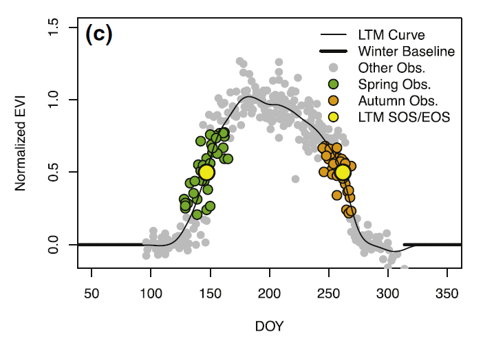
Figure 2. Example of LPA results for a sample deciduous forest 30-m Landsat pixel. Normalized EVI with long-term mean spline curve, long-term mean (LTM) transition dates (yellow dots) and in annual SOS and EOS, (green and orange dots, respectively). From Melaas et al., (2016).
Detection of SOS was not always possible at every pixel in every year because of persistent cloud cover during the springtime at some sites in some years, especially in eastern boreal Canada, which tends to be quite cloudy. To overcome this constraint, SOS time series were analyzed based on data that were up-scaled to the MODIS grid at 500-m spatial resolution using the mean 30-m SOS in each 500-m cell in each year. To ensure robust estimation of trends, 500-m cells were excluded with fewer than five forested Landsat pixels or for which fewer than 10 years of SOS retrievals were available.
The resulting dataset included nearly 1.2 million 500-m cells, where each grid cell provided a unique time series of SOS between 1984 and 2013. Using these time series, SOS trends were evaluated by computing the Theil-Sen slope (Sen, 1968) to estimate the magnitude of long-term SOS change, and then identified grid cells with statistically significant trends (p < 0.05) using the Mann-Kendall test (Mann, 1945).
Refer to Melaas et al. (2018) for additional details.
Data Access
These data are available through the Oak Ridge National Laboratory (ORNL) Distributed Active Archive Center (DAAC).
Landsat-derived Spring and Autumn Phenology, Eastern US - Canadian Forests, 1984-2013
Contact for Data Center Access Information:
- E-mail: uso@daac.ornl.gov
- Telephone: +1 (865) 241-3952
References
Melaas, E. K., M. A. Fridel, and D. Sulla-Menashe. 2018. Multidecadal Changes and Interannual Variation in Springtime Phenology of North American Temperate and Boreal Deciduous Forests. Geophysical Research Letters. https://doi.org/10.1002/2017GL076933
Melaas, E. K., Sulla-Menashe, D., Gray, J. M., Black, T. A., Morin, T. H., Richardson, A. D., & Friedl, M. A. (2016). Multisite analysis of land surface phenology in North American temperate and boreal deciduous forests from Landsat. Remote Sensing of Environment, 186, 452–464. https://doi.org/10.1016/j.rse.2016.09.014
Melaas, E. K., M.A. Friedl, M. A., and Zhu, Z. (2013). Detecting interannual variation in deciduous broadleaf forest phenology using Landsat TM/ETM + data. Remote Sensing of Environment, 132, 176–185. https://doi.org/10.1016/j.rse.2013.01.011
Sen, P. K. (1968). Estimates of the Regression Coefficient Based on Kendall’s Tau. Journal of the American Statistical Association, 63(324), 1379–1389. https://doi.org/10.1080/01621459.1968.10480934
Wulder, M. A., White, J. C., Cranny, M., Hall, R. J., Luther, J. E., Beaudoin, A., Goodenough, D.G., and Dechka, J. A. (2008). Monitoring Canada’s forests. Part 1: Completion of the EOSD land cover project. Canadian Journal of Remote Sensing, 34(6), 549–562. https://doi.org/10.5589/m08-066
Xian, G., Homer, C., & Fry, J. (2009). Updating the 2001 National Land Cover Database land cover classification to 2006 by using Landsat imagery change detection methods. Remote Sensing of Environment, 113(6), 1133–1147. https://doi.org/10.1016/j.rse.2009.02.004
Zhu, Z., & Woodcock, C. E. (2014). Continuous change detection and classification of land cover using all available Landsat data. Remote Sensing of Environment, 144, 152–171. https://doi.org/10.1016/j.rse.2014.01.011