Documentation Revision Date: 2019-09-19
Dataset Version: 1
Summary
The data products, consisting of almost 750 site-years of observations, can be used for phenological model validation and development, evaluation of satellite remote sensing data products, to understand relationships between canopy phenology and ecosystem processes, to study the seasonal changes in leaf-level physiology that are associated with changes in leaf color, for benchmarking earth system models, and for studies of climate change impacts on terrestrial ecosystems.
This data set contains 133 network site descriptions files (in both *.txt format and *.JSON format), 1082 region-of-interest definition (ROI) files in TIFF format, 1082 sample images for each image mask file in .jpg format and 1224 *.csv files, including ROI index files, and time series of extracted image color and greenness transitions processed to 1- and 3-day intervals.
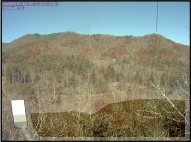
Figure 1. PhenoCam Network image from the Coweeta, North Carolina site. The region of interest (ROI) at the time this image was acquired was the transparent area with deciduous vegetation in the foreground.
Citation
Richardson, A.D., K. Hufkens, T. Milliman, D.M. Aubrecht, M. Chen, J.M. Gray, M.R. Johnston, T.F. Keenan, S.T. Klosterman, M. Kosmala, E.K. Melaas, M.A. Friedl, S. Frolking, M. Abraha, M. Alber, M. Apple, B.E. Law, D. Baldocchi, T.A. Black, P. Blanken, D.M. Browning, S. Bret-Harte, N. Brunsell, S.P. Burns, E. Cremonese, A.R. Desai, A.L. Dunn, D.M. Eissenstat, S.E. Euskirchen, L.B. Flanagan, B. Forsythe, J. Gallagher, L. Gu, D.Y. Hollinger, J.W. Jones, J. King, O. Langvall, J.H. McCaughey, P.J. McHale, G.A. Meyer, M.J. Mitchell, M. Migliavacca, Z. Nesic, A. Noormets, K. Novick, J. O'Connell, A.C. Oishi, W.W. Oswald, T.D. Perkins, R.P. Phillips, M.D. Schwartz, R.L. Scott, O. Sonnentag, J.E. Thom, and J. Verfaillie. 2018. PhenoCam Dataset v1.0: Vegetation Phenology from Digital Camera Imagery, 2000-2015. ORNL DAAC, Oak Ridge, Tennessee, USA. https://doi.org/10.3334/ORNLDAAC/1511
Table of Contents
- Dataset Overview
- Data Characteristics
- Application and Derivation
- Quality Assessment
- Data Acquisition, Materials, and Methods
- Data Access
- References
Dataset Overview
This data set provides time series of vegetation phenological observations for 133 sites across diverse ecosystems of North America and Europe from 2000-2015. The phenology data were derived from conventional visible-wavelength automated digital camera imagery collected through the PhenoCam Network at each site. From each acquired image, RGB (red, green, blue) color channel information was extracted and means and other statistics calculated for a region-of-interest (ROI) that delineates an area of specific vegetation type. From the high-frequency (typically, 30 minute) imagery collected over several years, time series characterizing vegetation color, including canopy greenness, plus greenness rising and greenness falling transition dates, were summarized over 1- and 3-day intervals.
The data products, consisting of almost 750 site-years of observations, can be used for phenological model validation and development, evaluation of satellite remote sensing data products, to understand relationships between canopy phenology and ecosystem processes, to study the seasonal changes in leaf-level physiology that are associated with changes in leaf color, for benchmarking earth system models, and for studies of climate change impacts on terrestrial ecosystems.
Related Publication with Full Documentation:
Please refer to, and cite, the following publication when you cite this dataset:
Richardson, A.D., Hufkens, K., Milliman, T., Aubrecht, D.M., Chen, M., Gray, J.M., Johnston, M.R., Keenan, T.F., Klosterman, S.T., Kosmala, M., Melaas, E.K., Friedl, M.A., Frolking, S. 2018. Tracking vegetation phenology across diverse North American biomes using PhenoCam imagery. Scientific Data 180028. DOI: https://doi.org/10.1038/sdata.2018.28
Related Dataset:
Milliman, T., K. Hufkens, A.D. Richardson, D.M. Aubrecht, M. Chen, J.M. Gray, M.R. Johnston, T. Keenan, S.T. Klosterman, M. Kosmala, E.K. Melaas, M.A. Friedl, S. Frolking, M. Abraha, M. Alber, M. Apple, B.E. Law, T.A. Black, P. Blanken, D. Browning, S. Bret-Harte, N. Brunsell, S.P. Burns, E. Cremonese, A.R. Desai, A.L. Dunn, D.M. Eissenstat, S.E. Euskirchen, L.B. Flanagan, B. Forsythe, J. Gallagher, L. Gu, D.Y. Hollinger, J.W. Jones, J. King, O. Langvall, J.H. McCaughey, P.J. McHale, G.A. Meyer, M.J. Mitchell, M. Migliavacca, Z. Nesic, A. Noormets, K. Novick, J. O'Connell, A.C. Oishi, W.W. Oswald, T.D. Perkins, R.P. Phillips, M.D. Schwartz, R.L. Scott, O. Sonnentag, and J.E. Thom. 2017. PhenoCam Dataset v1.0: Digital Camera Imagery from the PhenoCam Network, 2000-2015. ORNL DAAC, Oak Ridge, Tennessee, USA. https://doi.org/10.3334/ORNLDAAC/1560
Acknowledgments:
The development of PhenoCam has been funded by the Northeastern States Research Cooperative, NSF’s Macrosystems Biology program (awards EF-1065029 and EF-1702697), and DOE’s Regional and Global Climate Modeling program (award DE-SC0016011). We acknowledge additional support from the US National Park Service Inventory and Monitoring Program and the USA National Phenology Network (grant number G10AP00129 from the United States Geological Survey), and from the USA National Phenology Network and North Central Climate Science Center (cooperative agreement number G16AC00224 from the United States Geological Survey).
Data Characteristics
Spatial Coverage: Multiple points mostly over North America, some sites in Panama, Hawaii, and Europe
Spatial Resolution: Point
Temporal Resolution: half-hourly, daily and 3 days
Temporal Coverage: 1999-11-16 to 2017-03-03
Spatial Extent: (All latitude and longitude given in decimal degrees)
|
Sites |
Westernmost Longitude |
Easternmost Longitude |
Northernmost Latitude |
Southernmost Latitude |
|---|---|---|---|---|
|
Global |
-156.6091 |
34.8329 |
71.2801 |
9.154 |
Data File Information
File organization and data access
As described in the paper by Richardson et al. (2017), the PhenoCam Dataset v1.0 consists of a set of 5 data records for each site. The data can be accessed directly in the ORNL DAAC data pool at https://daac.ornl.gov/data/global_vegetation/PhenoCam_V1/ (after login).
Files in the data pool are organized as follows.
data_record_1 (contains general metadata for each site)
- <sitename>_meta.json
- <sitename>_meta.txt
data_record_2 (contains the ROI list files and image mask files used for image processing)
- <sitename>_<veg_type>_<ROI_ID_number>_roi.csv
- <sitename>_<veg_type>_<ROI_ID_number>_<mask_index>.tif
data_record_3 (contains time series of ROI color statistics, calculated for each image in the archive, using data_record_2)
- <sitename>_<veg_type>_<ROI_ID_number>_roistats.csv
data_record_4 (contains time series of ROI color summary statistics, calculated for 1 and 3 day aggregation periods from data_record_3)
- <sitename>_<veg_type>_<ROI_ID_number>_1day.csv
- <sitename>_<veg_type>_<ROI_ID_number>_3day.csv
data_record_5 (contains phenological transition dates, calculated from data_record_4)
- <sitename>_<veg_type>_<ROI_ID_number>_1day_ transition_dates.csv
- <sitename>_<veg_type>_<ROI_ID_number>_3day_transition_dates.csv
Here, <sitename> is the name of each camera site, <veg_type> is a two-letter code defining the type of vegetation for which data have been processed, and <ROI_ID_number> is a unique identifier to distinguish between multiple ROIs (regions of interest of the same vegetation type for a given site.
The Phenocam data can also be downloaded from the dataset landing page (https://daacdataset.ornl.gov/cgi-bin/dsviewer.pl?ds_id=1511), where all 3654 data files are presented without the directory structure mentioned above. Specific sites or data file types can be selected using the filter box at the top right of the data file list. For example, all 22 data files for the Acadia National Park site in Maine can be retrieved by typing "acadia" in the filter box, checking the checkbox for "Select All" , and clicking on the "Add Checked Items" button below the table. The data files will then be delivered using the ORNL DAAC Shopping Cart.
data_record_1: PhenoCam network site descriptions
These files provide general metadata for the PhenoCam network sites from which processed imagery has been included in this data set. Following general project information, site specific location, contacts, date range, and environmental and ecological characteristics are listed. The fields are specified as key-value pairs.
There are 133 sites (files) in standard text format (*.txt) and named as: <sitename>_meta.txt where sitename is the name of the respective camera site, e.g., acadia_meta.txt. The 133 machine-readable JSON files are named as <sitename>_meta.json.
The variables within the text files are as follows:
|
Column |
Description |
|---|---|
|
last_updated |
the date (format: YYYY-MM-DD, where MM = 01-12 and DD = 01-31) on which the site metadata were last updated |
|
project |
by default, all sites are associated with the PhenoCam Network project |
|
project_url |
the URL of the PhenoCam project web page |
|
fairuse_statement |
the general PhenoCam statement on data use, acknowledgment, and redistribution |
|
project_fairuse_url |
the URL of the PhenoCam fairuse_statement |
|
sitename |
the name of the camera site, e.g. “coweeta,” used to designate all images and products associated with that site |
|
long_name |
a more descriptive name for each camera site |
|
lat |
the latitude (in decimal degrees) of the camera itself |
|
lon |
the longitude (in decimal degrees) of the camera itself |
|
elevation |
the elevation of the ground surface (m above sea level) at the camera site |
|
contact1, contact2 |
the names and email addresses of the site representatives |
|
active |
“True” if new images from the site are still being added (as of last_updated date of the metadata file) to the PhenoCam archive; “False” otherwise |
|
date_start |
the date of the first image in the archive for this site |
|
date_end |
the date of the most recent image (as of the last_updated date of the metadata file) in the archive for this site (format: YYYY-MM-DD) |
|
nimage |
number of images in the archive for this site |
|
site_type |
the site class (Type I, II, or III) |
|
ir_enabled |
“Y” if the camera is capable of taking both visible and infrared (or visible+infrared) imagery |
|
method |
sites for which images are pushed to the PhenoCam server via FTP are designated “ftppush”, those for which images are pulled from an external server are designated “httppull” |
|
utc_offset |
the difference (in hours) between UTC (Coordinated Universal Time) and standard time at the site |
|
camera_description |
the brand and model of the camera being used |
|
camera_orientation |
the compass direction in which the camera is pointing |
|
group |
a number of camera sub-networks |
|
flux_data |
“True” if eddy covariance flux measurements are being (or have been) made at the site |
|
flux_networks |
if the site belongs to a network (e.g., AmeriFlux, Fluxnet-Canada, etc.), then the network is identified |
|
flux_sitenames |
FLUXNET site code, if applicable |
|
ecoregion |
numeric code identifying the site’s EPA Ecoregion |
|
MAP_site |
mean annual precipitation (mm) as reported by site personnel |
|
MAP_daymet |
mean annual precipitation (mm) from the Daymet |
|
MAP_worldclim |
mean annual precipitation (mm) from WorldClim |
|
MAT_site |
mean annual temperature (°C) as reported by site personnel |
|
MAT_daymet |
mean annual temperature (°C) from the Daymet |
|
MAT_worldclim |
mean annual temperature (°C) from WorldClim |
|
primary_veg_type |
the dominant vegetation type at the site |
|
secondary_veg |
secondary vegetation type at the site |
|
dominant_species |
Latin binomials for the dominant species at each site, as reported by site personnel |
|
landcover_igbp |
numeric code corresponding to the land cover classification scheme of the International Geosphere-Biosphere Programme, as derived from MODIS remote sensing Friedl et. al., 2010, Channan et al., 2014) |
|
wwf_biome |
numeric code corresponding to the biome classification scheme of the World Wildlife Fund (Olson et al., 2001) |
|
koeppen_geiger |
climate classification according to the Köppen-Geiger system (Kottek et al, 2006) |
|
site_acknowledgments |
data end users are asked to include this text, which has been provided by site collaborators, in publications and presentations that make use of data for this site |
data_record_2: ROI (Region of Interest) files
These files provide (1) the “ROI list files”, which detail the date and time range over which each binary image mask was applied in processing the image data for a site; and (2) the binary “image mask file”, which delineate the ROI over which the image analysis was conducted and (3) sample images for each image mask file. With (1) and (2) the data presented in the *_roistats.csv data files can be reproduced from the original image files.
There are 204 *_roi.csv ROI list files named as: <sitename>_<veg_type>_<ROI_ID_number>_roi.csv
Where <sitename> is the name of the network camera site, <veg_type> is a two-letter abbreviation identifying the dominant vegetation within the ROI, e.g. DB for deciduous broadleaf trees (see Table 1), and <ROI_ID_number> is a numeric code that serves as a unique identifier to distinguish between multiple ROIs of the same vegetation type at a given site (0001 for the first ROI list, 0002 for the second, etc.).
The first 13 lines (beginning with #), document the provenance of the ROI list, and contain a brief description of the vegetation that is delineated by the associated image masks. Line 14 lists the column headers for the mask entry rows.
|
Note that only images within the date and time ranges (from start_date and start_time to end_date and end_time) listed are included in the processed data set generated from this list. For end_date, the date code 9999-12-31 is used to keep the processing open-ended. |
The column descriptions are as follows:
|
Column |
Description |
|---|---|
|
start_date |
the date of the first image in the archive for this site |
|
start_time |
the time of capture of the first image for this site |
|
end_date |
the date of the most recent image (as of the last_updated date of the metadata file) in the archive for this site (format: YYYY-MM-DD) |
|
end_time |
the time of capture of the most recent image for this site |
|
mask_file |
the filename for the 8-bit TIFF mask file with black for the ROI and white for the region to exclude from calculations |
|
sample_image |
the filename for a sample image in the date range |
ROI (Region of Interest) Mask and Image Files:
These are the binary “image mask files”, which delineate the ROI (black for the ROI and white for the region to exclude from calculations) over which the image analysis was conducted.
There are 1082 files in TIFF (*.tif) format and are named as <sitename>_<veg_type>_<ROI_ID_number>_<mask_index>.tif .
Where <sitename> is the name of the network camera site and veg_type is a two-letter abbreviation identifying the dominant vegetation within the ROI, e.g. DB for deciduous broadleaf trees,
ROI_ID_number is a numeric code that serves as a unique identifier to distinguish between multiple ROIs of the same vegetation type at a given site (0001 for the first ROI list, 0002 for the second, etc.) and the
mask_index matches the entry number in the list (01 for the first entry, 02 for the second entry, etc.).
For example, acadia_DB_0001_01.tif, …, acadia_DB_0001_07.tif
The 1082 sample images for each mask file have the same naming convention but terminate in a .jpg extension:
<sitename>_<veg_type>_<ROI_ID_number>_<mask_index>.jpg
Vegetation-type abbreviations for ROIs
Vegetation type abbreviations for ROIs (region of interests).
|
Abbreviation |
Description |
|---|---|
|
AG |
agriculture |
|
DB |
deciduous broadleaf |
|
DN |
deciduous needleleaf |
|
EB |
evergreen broadleaf |
|
EN |
evergreen needleleaf |
|
GR |
grassland |
|
MX |
mixed vegetation |
|
SH |
shrubs |
|
TN |
tundra |
|
WT |
wetland |
|
NV |
non-vegetated |
|
RF |
reference panel |
|
XX |
unspecified |
data_record_3: Time Series of Color Information Extracted for Each ROI/Site Pair
These files contain the high-frequency (typically, 30 minute) color information extracted from the entire image archive for each site, using the ROI list files and image mask files note in the previous described data files.
For each archived image, RGB (red, green, blue) color channel information, with means and other statistics calculated across a region-of-interest (ROI) delineating a specific vegetation type was extracted. From the high-frequency (typically, 30 minute) imagery, time series characterizing vegetation color, including “canopy greenness”.
The providers refer to these as the “ROI statistics” time series files. The time series have not been filtered, and each data row in the file corresponds to an individual image in the archive.
There are 204 “ROI statistics” time series files named as <sitename>_<veg_type>_<ROI_ID_number>_roistats.csv
Where sitename, veg_type, and ROI_ID_number are the same as previous described.
File description for time series files:
The first 17 lines (beginning with #) contain basic metadata:
Line 4 contains the sitename, identical to that in the filename.
Lines 5 (veg_type) and 6 (ROI_ID_number) identify the vegetation type and the ROI_ID from the ROI list files.
Lines 7-9 are site location (latitude and longitude in decimal degrees, and elevation in m above sea level.
Line 10 is the UTC offset. [Lines 4-10 were extracted from the site metadata text files.]
Line 11 indicates whether images have been re- resized to common dimensions (to match the size of the mask file) prior to analysis.
Line 12 indicates the version of the data set.
Lines 13-16 document the provenance of the data file.
Line 18 lists the column headers for the data rows.
The data rows begin on line 19 with each data row corresponding to results for an individual image in the archive.
The column descriptions are as follows:
|
Column |
Description |
|---|---|
|
date |
local date |
|
local_std_time |
local standard time |
|
doy |
day of year |
|
filename |
image filename |
|
solar_elev |
solar elevation angle, in degrees |
|
exposure |
image exposure |
|
mask_index |
mask number in the image mask sequence |
|
gcc |
mean green chromatic coordinate (Gcc) over the ROI |
|
rcc |
mean red chromatic coordinate (Rcc) over the ROI |
|
r_mean |
mean red channel DN over the ROI |
|
r_std |
standard deviation (across pixels) of red channel DN over the ROI |
|
b_mean |
mean blue channel DN over the ROI |
|
b_std |
standard deviation (across pixels) of blue channel DN over the ROI |
|
g_mean |
mean green channel DN over the ROI |
|
g_std |
standard deviation (across pixels) of green channel DN over the ROI |
|
r_5_qtl |
the 5th quantile values (across pixels) of the red channel DN over the ROI |
|
r_10_qtl |
the 10th quantile values (across pixels) of the red channel DN over the ROI |
|
r_25_qtl |
the 25th quantile values (across pixels) of the red channel DN over the ROI |
|
r_50_qtl |
the 50th quantile values (across pixels) of the red channel DN over the ROI |
|
r_75_qtl |
the 75th quantile values (across pixels) of the red channel DN over the ROI |
|
r_90_qtl |
the 90th quantile values (across pixels) of the red channel DN over the ROI |
|
r_95_qtl |
the 95th quantile values (across pixels) of the red channel DN over the ROI |
|
b_5_qtl |
the 5th quantile values (across pixels) of the blue channel DN over the ROI |
|
b_10_qtl |
the 10th quantile values (across pixels) of the blue channel DN over the ROI |
|
b_25_qtl |
the 25th quantile values (across pixels) of the blue channel DN over the ROI |
|
b_50_qtl |
the 50th quantile values (across pixels) of the blue channel DN over the ROI |
|
b_75_qtl |
the 75th quantile values (across pixels) of the blue channel DN over the ROI |
|
b_90_qtl |
the 90th quantile values (across pixels) of the blue channel DN over the ROI |
|
b_95_qtl |
the 95th quantile values (across pixels) of the blue channel DN over the ROI |
|
g_5_qtl |
the 5th quantile values (across pixels) of the green channel DN over the ROI |
|
g_10_qtl |
the 10th quantile values (across pixels) of the green channel DN over the ROI |
|
g_25_qtl |
the 25th quantile values (across pixels) of the green channel DN over the ROI |
|
g_50_qtl |
the 50th quantile values (across pixels) of the green channel DN over the ROI |
|
g_75_qtl |
the 75th quantile values (across pixels) of the green channel DN over the ROI |
|
g_90_qtl |
the 90th quantile values (across pixels) of the green channel DN over the ROI |
|
g_95_qtl |
the 95th quantile values (across pixels) of the green channel DN over the ROI |
|
r_g_cor |
correlation coefficient (across pixels) between red channel DN and green channel DN, over the ROI |
|
g_b_cor |
correlation coefficient between green channel DN and blue channel DN, over the ROI |
|
b_r_cor |
correlation coefficient between blue channel DN and red channel DN, over the ROI |
data_record_4: 1- Day and 3- day Summary Product Files
1- day summary product files:
These files contain the daily summaries of the high-frequency (typically, 30 minute) time series data characterizing vegetation color, including “canopy greenness” for each site.
As noted previously, for each archived image, RGB (red, green, blue) color channel information, with means and other statistics calculated across a region-of-interest (ROI) delineating a specific vegetation type was extracted. From the high-frequency (typically, 30 minute) imagery, time series characterizing vegetation color, including “canopy greenness” was processed to 1-day intervals.
There are 204 1-day summary product files named as <sitename>_<veg_type>_<ROI_ID_number>_1day.csv. Where sitename, veg_type, and ROI_ID_number are the same as previous described.
File description for 1- day summary product files:
The first 24 lines (beginning with #) contain basic metadata.
Lines 4 through 10 are identical to those in the all-image time series file from which the summary product files are derived.
Line 11 is not used in the data sets but allows for the specification of an image count threshold for processing to occur (i.e., if for a given period of aggregation, there are insufficient images available, then only results for the midday image, if applicable, would be reported).
Line 12 gives the number of days that have been aggregated in producing the file, which is 1 day.
Line 13 reports the solar elevation filter that was used in processing (10° in the current data set).
Lines 14 and 15 are not used in the data sets but allows for the specification of time-of-day window (i.e., images outside of the window would be excluded from the processing).
Lines 16 and 17 report the values that were used for the “too dark” and “too bright” quality control filters, which are by default set to DN 100 and 665, respectively. Lines 18-23 document the provenance of the data file. Line 25 lists the column headers for the data rows.
The data rows begin on line 26, and for each data row the data fields are:
|
Column |
Description |
|---|---|
|
date |
local date at the middle of the aggregation period (1-day) |
|
year |
calendar year of the above date (YYYY) |
|
doy |
day of year for the above date |
|
image_count |
the number of images passing the selection criteria |
|
midday_filename |
the filename of the image which is closest to 12 noon |
|
midday_r |
mean red channel DN over the ROI, for the midday image |
|
midday_g |
mean green channel DN over the ROI, for the midday image |
|
midday_b |
mean blue channel DN over the ROI, for the midday image |
|
midday_gcc |
the mean GCC over the ROI, for the midday image |
|
midday_rcc |
the mean RCC over the ROI, for the midday image |
|
r_mean |
the mean value (for all images passing the selection criteria) of the mean (by image) red channel DN over the ROI |
|
r_std |
the standard deviation (for all images passing the selection criteria) of the mean (by image) red channel DN over the ROI |
|
g_mean |
the mean value (for all images passing the selection criteria) of the mean (by image) green channel DN over the ROI |
|
g_std |
the standard deviation (for all images passing the selection criteria) of the mean (by image) green channel DN over the ROI |
|
b_mean |
the mean value (for all images passing the selection criteria) of the mean (by image) blue channel DN over the ROI |
|
b_std |
the standard deviation (for all images passing the selection criteria) of the mean (by image) blue channel DN over the ROI |
|
gcc_mean |
the mean value (for all images passing the selection criteria) of the mean (by image) Gcc over the ROI |
|
gcc_std |
the standard deviation (for all images passing the selection criteria) of the mean (by image) Gcc over the ROI |
|
gcc_50, gcc_75, gcc_90 |
the 50th, 75th and 90th quantiles (for all images passing the selection criteria) of the mean (by image) GCC over the ROI |
|
rcc_mean, rcc_std, rcc_50, rcc_75, rcc_90 |
the 50th, 75th and 90th quantiles (for all images passing the selection criteria) of the mean (by image) RGCC over the ROI |
|
max_solar_elev |
the maximum solar elevation angle for all images passing the selection criteria |
|
snowflag |
a citizen-science based evaluation of the presence of snow in the midday image. The snowflag is coded as follows: 1 = bad or obscured image; 2 = no snow in image; 3 = snow on ground (used for non-tree sites); 4 = snow on ground only (used for treed sites); 5 = snow on trees (and ground; used for treed sites). If the midday image was not evaluated, a value of NA is assigned. |
|
outlierflag_gcc_mean, outlierflag_gcc_50; outlierflag_gcc_75, outlierflag_gcc_90 |
the outlierflag, which is determined separately for the gcc_mean, gcc_50, gcc_75, and gcc_90 time series, can either take on a value of 0 (indicating good data), or 1 (indicating an outlier) |
|
smooth_gcc_mean, smooth_gcc_50, smooth_gcc_75, smooth_gcc_90 |
the smoothed and/or interpolated value of Gcc from the final iteration (i.e. with outliers removed) of the spline fitting process |
|
smooth_rcc_mean, smooth_rcc_50, smooth_rcc_75, smooth_rcc_90 |
the smoothed and/or interpolated value of Rcc from the final iteration (i.e. with outliers removed) of the spline fitting process |
|
smooth_ci_gcc_mean, smooth_ci_gcc_50, smooth_ci_gcc_75, smooth_ci_gcc_90 |
the (one-sided) width of the 95% confidence interval around the smoothed GCC values |
|
smooth_ci_rcc_mean, smooth_ci_rcc_50, smooth_ci_rcc_75, smooth_ci_rcc_90 |
the (one-sided) width of the 95% confidence interval around the smoothed RCC values |
|
int_flag |
to assist with identification of long gaps in the data record, the interpolation flag is set to 1 during a gap of 14 days or more |
3- Day Summary Product Files
These files contain the 3-day summaries of the high-frequency (typically, 30 minute) time series data characterizing vegetation color, including “canopy greenness” for each site.
As noted previously, for each archived image, RGB (red, green, blue) color channel information, with means and other statistics calculated across a region-of-interest (ROI) delineating a specific vegetation type was extracted. From the high-frequency (typically, 30 minute) imagery, time series characterizing vegetation color, including “canopy greenness” was processed to 3-day intervals.
There are 204 3-day summary product files named as <sitename>_<veg_type>_<ROI_ID_number>_3day.csv. Where sitename, veg_type, and ROI_ID_number are the same as previous described.
File description for 3-day summary product files:
The first 24 lines (beginning with #) contain basic metadata.
Lines 4 through 10 are identical to those in the all-image time series file from which the summary product files are derived.
Line 11 is not used in the data sets but allows for the specification of an image count threshold for processing to occur (i.e., if for a given period of aggregation, there are insufficient images available, then only results for the midday image, if applicable, would be reported).
Line 12 gives the number of days that have been aggregated in producing the file, which is 3 days.
Line 13 reports the solar elevation filter that was used in processing (10° in the current data set).
Lines 14 and 15 are not used in the data sets but allows for the specification of time-of-day window (i.e., images outside of the window would be excluded from the processing).
Lines 16 and 17 report the values that were used for the “too dark” and “too bright” quality control filters, which are by default set to DN 100 and 665, respectively.
Lines 18-23 document the provenance of the data file.
Line 25 lists the column headers for the data rows.
The data rows begin on line 26, and for each data row the data fields are:
|
Column |
Description |
|---|---|
|
date |
local date at the middle of the aggregation period ( 3-day) |
|
year |
calendar year of the above date (YYYY) |
|
doy |
day of year for the above date |
|
image_count |
the number of images passing the selection criteria |
|
midday_filename |
the filename of the image which is closest to 12 noon |
|
midday_r |
mean red channel DN over the ROI, for the midday image |
|
midday_g |
mean green channel DN over the ROI, for the midday image |
|
midday_b |
mean blue channel DN over the ROI, for the midday image |
|
midday_gcc |
the mean GCC over the ROI, for the midday image |
|
midday_rcc |
the mean RCC over the ROI, for the midday image |
|
r_mean |
the mean value (for all images passing the selection criteria) of the mean (by image) red channel DN over the ROI |
|
r_std |
the standard deviation (for all images passing the selection criteria) of the mean (by image) red channel DN over the ROI |
|
g_mean |
the mean value (for all images passing the selection criteria) of the mean (by image) green channel DN over the ROI |
|
g_std |
the standard deviation (for all images passing the selection criteria) of the mean (by image) green channel DN over the ROI |
|
b_mean |
the mean value (for all images passing the selection criteria) of the mean (by image) blue channel DN over the ROI |
|
b_std |
the standard deviation (for all images passing the selection criteria) of the mean (by image) blue channel DN over the ROI |
|
gcc_mean |
the mean value (for all images passing the selection criteria) of the mean (by image) Gcc over the ROI |
|
gcc_std |
the standard deviation (for all images passing the selection criteria) of the mean (by image) Gcc over the ROI |
|
gcc_50, gcc_75, gcc_90 |
the 50th, 75th and 90th quantiles (for all images passing the selection criteria) of the mean (by image) GCC over the ROI |
|
rcc_mean, rcc_std, rcc_50, rcc_75, rcc_90 |
the 50th, 75th and 90th quantiles (for all images passing the selection criteria) of the mean (by image) RGCC over the ROI |
|
max_solar_elev |
the maximum solar elevation angle for all images passing the selection criteria |
|
snowflag |
a citizen-science based evaluation of the presence of snow in the midday image. The snowflag is coded as follows: 1 = bad or obscured image; 2 = no snow in image; 3 = snow on ground (used for non-tree sites); 4 = snow on ground only (used for treed sites); 5 = snow on trees (and ground; used for treed sites). If the midday image was not evaluated, a value of NA is assigned. |
|
outlierflag_gcc_mean, outlierflag_gcc_50; outlierflag_gcc_75, outlierflag_gcc_90 |
the outlierflag, which is determined separately for the gcc_mean, gcc_50, gcc_75, and gcc_90 time series, can either take on a value of 0 (indicating good data), or 1 (indicating an outlier) |
|
smooth_gcc_mean, smooth_gcc_50, smooth_gcc_75, smooth_gcc_90 |
the smoothed and/or interpolated value of Gcc from the final iteration (i.e. with outliers removed) of the spline fitting process |
|
smooth_rcc_mean, smooth_rcc_50, smooth_rcc_75, smooth_rcc_90 |
the smoothed and/or interpolated value of Rcc from the final iteration (i.e. with outliers removed) of the spline fitting process |
|
smooth_ci_gcc_mean, smooth_ci_gcc_50, smooth_ci_gcc_75, smooth_ci_gcc_90 |
the (one-sided) width of the 95% confidence interval around the smoothed GCC values |
|
smooth_ci_rcc_mean, smooth_ci_rcc_50, smooth_ci_rcc_75, smooth_ci_rcc_90 |
the (one-sided) width of the 95% confidence interval around the smoothed RCC values |
|
int_flag |
to assist with identification of long gaps in the data record, the interpolation flag is set to 1 during a gap of 14 days or more |
data_record_5: Greenness Transition Date Estimate Files
These data files contain the transition date estimates for the start of each “greenness rising” stage and end of each “greenness falling” stage, derived from the 1-day and 3-day summary data.
There are 408 transition date files.
The transition date files are named as:
<sitename>_<veg_type>_<ROI_ID_number>_1day_ transition_dates.csv, and <sitename>_<veg_type>_<ROI_ID_number>_3day_transition_dates.csv
Where <sitename> is the name of the network camera site, <veg_type> is a two-letter abbreviation identifying the dominant vegetation within the ROI, e.g. DB for deciduous broadleaf trees (see Table 1), and <ROI_ID_number> is a numeric code that serves as a unique identifier to distinguish between multiple ROIs of the same vegetation type at a given site (0001 for the first ROI list, 0002 for the second, etc.).
File description for transition date files:
The first 16 lines (beginning with #) contain basic metadata.
Lines 4 through 6 are identical to those in the summary product file from which the transition date file is derived.
Line 7 gives the number of days that have been aggregated in producing the file, which is either 1 day (if transition dates are calculated from Data Record 4) or 3 days (if transition dates are calculated from Data Record 5).
Lines 8 and 9 define the first and last years for which the transition dates are calculated.
Lines 10 and 11 document the provenance of the data file.
Lines 12-15 report goodness-of-fit statistics (in terms of RMSE, the root mean squared error) for the spline curves from which the transition dates are extracted.
Line 17 lists the column headers for the data rows.
The data rows begin on line 18, and for each data row, corresponding to a single “greenness rising” or “greenness falling” stage.
|
Column |
Description |
|---|---|
|
sitename |
the name of the camera site |
|
veg_type |
a two-letter abbreviation identifying the dominant vegetation within the ROI |
|
roi_id |
a numeric code (ROI_ID_number) to distinguish between multiple ROIs of the same vegetation type at a given site |
|
direction |
indicates whether the reported transition dates correspond to a “greenness rising” or “greenness falling” stage. Note that there may be more than one rising/falling cycle per calendar year, and a single rising or falling stage may cut across years. |
|
gcc_value |
indicates whether the transition dates are calculated from gcc_mean, gcc_50, gcc_75 or gcc_90 time series (a typical file will include dates calculated for each of these) |
|
transition_10, transition_25, transition_50 |
the extracted transition dates (format YYYY-MM-DD) for each “greenness rising” or “greenness falling” stage, corresponding to 10%, 25% and 50% of the GCC amplitude of that stage |
|
transition_10_lower_ci, transition_25_lower_ci, transition_50_lower_ci, transition_10_upper_ci, transition_25_upper_ci, transition_50_upper_ci |
dates (format YYYY-MM-DD) corresponding to the lower and upper, respectively, 95% confidence intervals on the extracted transition dates (10%, 25%, and 50% of the GCC amplitude) |
|
threshold_10, threshold_25, threshold_50 |
the threshold values of GCC used to identify transition dates |
|
min_gcc, max_gcc |
the baseline (dormant-season minimum) and peak (active-season maximum) GCC values, calculated from the fitted spline, as used to derive the GCC amplitude |
Application and Derivation
Data derived from PhenoCam imageries can be used for phenological model validation and development, evaluation of satellite remote sensing data products, understand relationships between canopy phenology and ecosystem processes, to study the seasonal changes in leaf-level physiology that are associated with changes in leaf color, benchmarking earth system models, and studies of climate change impacts on terrestrial ecosystems (Richardson et al., 2017).
Quality Assessment
Quantitative analysis through automated quality control routines (e.g. filtering and outlier detection, described in Richardson et al., 2107) and visual evaluation of each time series has been vetted for consistency and overall quality (Richardson et al., 2017)
Data Acquisition, Materials, and Methods
Following are brief excerpts from Richardson et al. (2017). See this publication for more details.
PhenoCam Network
The PhenoCam network is a cooperative network, established in 2008 and uses digital camera imagery to monitor ecosystem dynamics over time. It serves as a long-term, continental-scale, phenological observatory with cameras deployed within North America, from Alaska to Texas, and from Maine to Hawaii (Figure 2), and some on other continents.
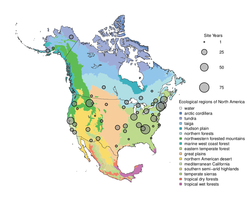
Figure 2: Spatial distribution of PhenoCam data across ecological regions of North America. Background map illustrates USA Environmental Protection Agency Level I Ecoregions. Data counts have been aggregated to a spatial resolution of 4°, and the size of each circle corresponds to the number of years of data. Sites in Hawaii, Panama, and Europe are not shown.
The data sets presented here are derived conventional, visible-wavelength, automated digital camera imagery from over 400 cameras, together totaling almost 750 years of data across different ecoregions, climate zones, and vegetation types. Vegetation types such as deciduous broadleaf forests (392 site-years of data in the dataset), grasslands (121 site-years), and evergreen needleleaf forests (80 site- years) are the best-represented. For each archived image, RGB (red, green, blue) color channel information, with means and other statistics calculated across a region-of-interest (ROI) delineating a specific vegetation type was extracted. From the high-frequency (typically, 30 minute) imagery, time series characterizing vegetation color, including canopy greenness (canopy greenness index -- the green chromatic coordinate, Gcc) processed to 1- and 3-day intervals was derived. For ecosystems with one or more annual cycles of vegetation activity, uncertainties, for the start of the “greenness rising” and end of the “greenness falling” stages has been provided. Every night, any new images that have been uploaded to the server during the previous 24 hours are copied to the data archive, and then processed and analysed as described in Richardson et. al., 2017. The processing is conducted using scripts coded in Python. The scripts used for image processing, including extraction of colour information, and generation of ‘all-image’ and ‘summary’ time series data product files, are available at https://github.com/tmilliman/python-vegindex/ with an open source license agreement.
Image analysis and data processing
Image analysis consists of several steps. First, an appropriate “region of interest” (ROI) is defined, corresponding to the area within each digital image for which color information will be extracted. The ROIs characterize the dominant vegetation type in each image. For sites where more than one vegetation type could be clearly identified, secondary ROIs are selected. The ROI coordinate definitions are stored, in TIFF format, as a series of binary image masks, which comprise an ROI’s “mask sequence”. For each ROI mask sequence at each site, an “ROI list file” detailing the date and time range over which each mask is to be applied.
The digital cameras record JPEG images with color information stored in three separate layers (red, green, and blue; RGB). According to the standard additive color model, representation of any given color in the visible range is achieved by varying the intensity (pixel value) of these primary colors. Thus, each pixel in the image is associated with a digital number (“DN”) triplet, with each element in the triplet corresponding to the intensity of one of the color layers. Therefore, the second step in the image analysis is to read in the images, and associated mask sequence, and to characterize the frequency distribution of the RGB DN triplets across the mask. This is done separately for each ROI at each site, to produce the “ROI statistics” time series data files.
For each image, the date and local time were extracted from the image file name. In addition, the solar elevation angle based on the date and local time stamp, using standard formulas is also calculated.
The frequency distribution of the RGB DN triplets across the mask was characterized on a channel-by-channel basis, and also in terms of the pairwise correlation of DN values between color channels. Thus, for each of the red, green and blue color channels, the mean and standard deviation, as well as the 5th, 10th, 25th, 50th, 75th, 90th, and 95th quantiles, of the DN distribution across all pixels in the ROI was determined.
Transition Date Estimation
Using an approach similar to the “spline interpolation” method that has been previously applied to PhenoCam data, phenophase transition dates for each ROI mask sequence has been extracted. These are intended to define the start of the “greenness rising” and end of the “greenness falling” stage for a full cycle of vegetation activity (i.e., from dormancy, through green-up or “greenness rising”, peak activity, senescence or “greenness falling”, and back to dormancy).
Data Access
These data are available through the Oak Ridge National Laboratory (ORNL) Distributed Active Archive Center (DAAC).
PhenoCam Dataset v1.0: Vegetation Phenology from Digital Camera Imagery, 2000-2015
Contact for Data Center Access Information:
- E-mail: uso@daac.ornl.gov
- Telephone: +1 (865) 241-3952
References
Channan, S., Collins, K. and Emanuel, W.R., 2014. Global mosaics of the standard MODIS land cover type data. University of Maryland and the Pacific Northwest National Laboratory, College Park, Maryland, USA, 30.
Friedl, M.A., Sulla-Menashe, D., Tan, B., Schneider, A., Ramankutty, N., Sibley, A. and Huang, X., 2010. MODIS Collection 5 global land cover: Algorithm refinements and characterization of new datasets. Remote sensing of Environment, 114(1), pp.168-182. https://doi.org/10.1016/j.rse.2009.08.016
Kottek, M., Grieser, J., Beck, C., Rudolf, B. and Rubel, F., 2006. World map of the Köppen-Geiger climate classification updated. Meteorologische Zeitschrift, 15(3), pp.259-263. https://doi.org/10.1127/0941-2948/2006/0130
Olson, D.M., Dinerstein, E., Wikramanayake, E.D., Burgess, N.D., Powell, G.V., Underwood, E.C., D'amico, J.A., Itoua, I., Strand, H.E., Morrison, J.C. and Loucks, C.J., 2001. Terrestrial Ecoregions of the World: A New Map of Life on Earth: A new global map of terrestrial ecoregions provides an innovative tool for conserving biodiversity. BioScience, 51(11), pp.933-938. https://doi.org/10.1641/0006-3568(2001)051[0933:TEOTWA]2.0.CO;2
Richardson, A.D., Hufkens, K., Milliman, T., Aubrecht, D.M., Chen, M., Gray, J.M., Johnston, M.R., Keenan, T.F., Klosterman, S.T., Kosmala, M., Melaas, E.K., Friedl, M.A., Frolking, S. 2018. Tracking vegetation phenology across diverse North American biomes using PhenoCam imagery. Scientific Data 180028. DOI: https://doi.org/10.1038/sdata.2018.28