Documentation Revision Date: 2023-09-27
Dataset Version: 1
Summary
This dataset contains 312 data files in cloud-optimized GeoTIFF format (LSP-EVI2 and LSP-Dates), one shapefile provided in a compressed .zip file, and one file in comma-separated values (.csv) format.
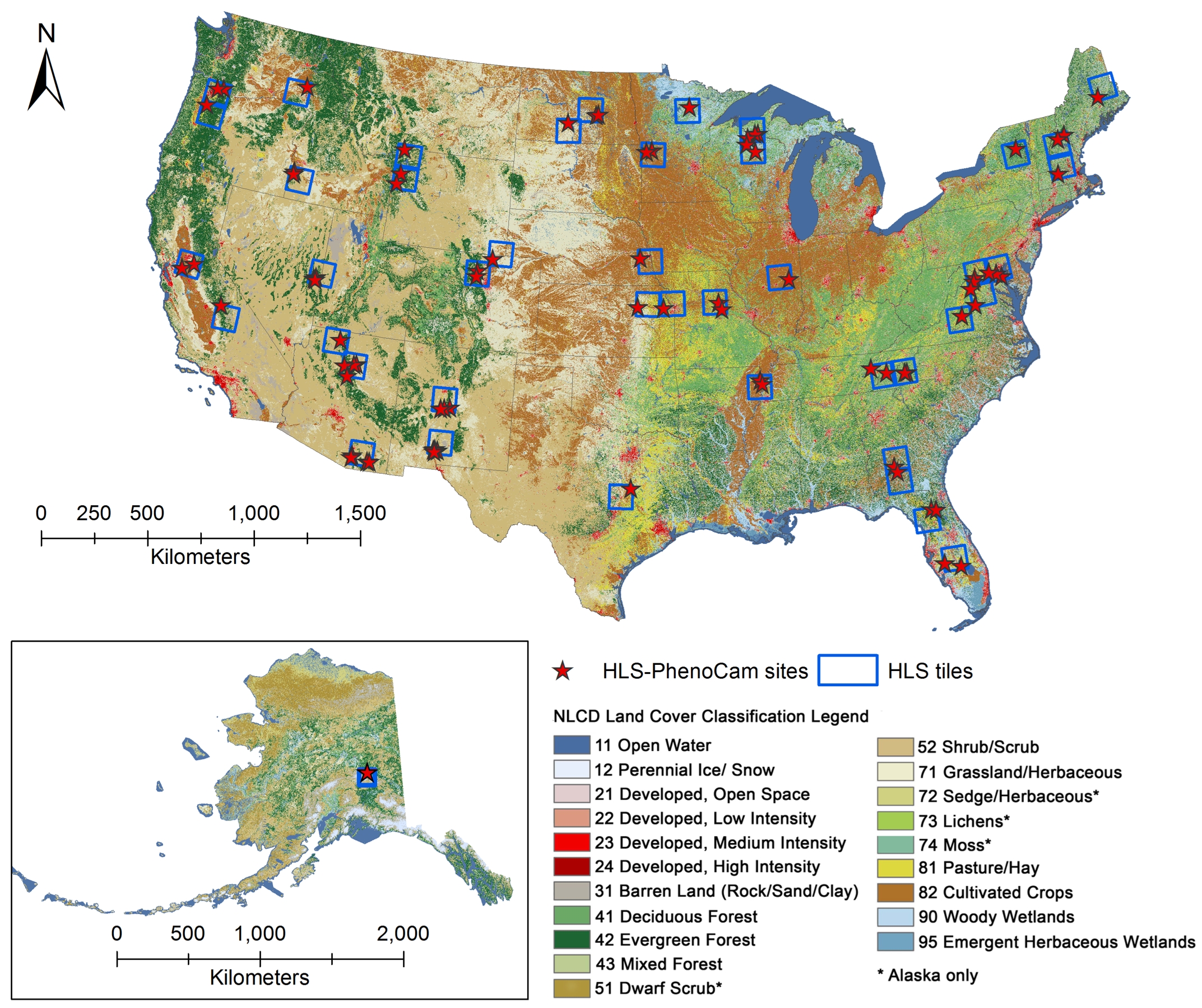
Figure 1. Geographical distribution of 78 regions included in the HLS-PhenoCam LSP dataset across various ecosystems in North America. Each region covers 10 x 10 km2 with at least one PhenoCam site. The background is the 30-m National Land Cover Database (NLCD) product displaying the land cover types (NLCD 2019 for CONUS and NLCD 2016 for Alaska).
Citation
Tran, K.H., X. Zhang, Y. Ye, Y. Shen, S. Gao, Y. Liu, and A.D. Richardson. 2023. Phenology derived from Satellite Data and PhenoCam across CONUS and Alaska, 2019-2020. ORNL DAAC, Oak Ridge, Tennessee, USA. https://doi.org/10.3334/ORNLDAAC/2248
Table of Contents
- Dataset Overview
- Data Characteristics
- Application and Derivation
- Quality Assessment
- Data Acquisition, Materials, and Methods
- Data Access
- References
Dataset Overview
The HLS-PhenoCam LSP (HP-LSP) dataset is a reference of vegetation phenology development at 30-m pixels that was produced by bridging the temporal HLS observations with near-surface PhenoCam time series. The dataset consists of 78 regions (each region covers 10 × 10 km2 with at least one PhenoCam site) across various plant functional types and climates in North America during 2019 and 2020, which leads to approximately 17 million samples with a spatial resolution of 30 m. The HP-LSP dataset includes two portions: (1) the 3-day synthetic gap-free HLS-PhenoCam EVI2 time series, and (2) spatially continuous and scalable phenometrics (greenup onset, maturity onset, senescence onset, and dormancy onset) with up to three vegetation growing cycles during a year.
The PhenoCam network offers near-surface observations via the RGB (Red, Green, and Blue) imagery without cloud contamination every 30 minutes. Each RGB imagery provides a tool to calculate as many as 100 Green Chromatic Coordinate (GCC), a proportional measure of the green band to the sum of all RGB channels, which enables us to create a collection of GCC time series for observing local vegetation dynamics. The HLS EVI2 time series with frequent gaps was fused with the most comparable PhenoCam GCC temporal shape selected from the GCC collection using the Spatiotemporal Shape Matching Model (SSMM) to generate the synthetic gap-free HLS-PhenoCam EVI2 time series, which was used to establish the physically-based hybrid piecewise logistic model (HPLM) that was then applied to detect the phenological transition dates (phenometrics).
The ORNL DAAC compiles, archives, and distributes data on vegetation from local to global scales. Specific topic areas include: belowground vegetation characteristics and roots, vegetation biomass, fire and other disturbance, vegetation dynamics, land cover and land use change, vegetation characteristics, and NPP (Net Primary Production) data.
Related publication
Tran, K.H., X. Zhang, Y. Ye, Y. Shen, S. Gao, Y. Liu, and A. Richardson. 2023. HP-LSP: A reference of land surface phenology from fused Harmonized Landsat and Sentinel-2 with PhenoCam data. Sci Data. (In process).
Tran, K.H., X. Zhang, A.R. Ketchpaw, J. Wang, Y. Ye, and Y. Shen. 2022. A novel algorithm for the generation of gap-free time series by fusing harmonized Landsat 8 and Sentinel-2 observations with PhenoCam time series for detecting land surface phenology. Remote Sensing of Environment 282:113275. https://doi.org/10.1016/j.rse.2022.113275.
Acknowledgement
This work was supported by NASA grants 80NSSC21K1962 and 80NSSC20K1337. The development of PhenoCam has been funded by the Northeastern States Research Cooperative, NSF's Macrosystems Biology program (awards EF-1065029 and EF-1702697), and DOE's Regional and Global Climate Modeling program (award DE-SC0016011).
Data Characteristics
Spatial Coverage: CONUS and Alaska
Spatial Resolution: 30 m
Temporal Coverage: 2019-01-01 - 2020-12-31
Study Area: Coordinates are provided in decimal degrees
| Site | Westernmost Longitude | Easternmost Longitude | Northernmost Latitude | Southernmost Latitude |
|---|---|---|---|---|
| CONUS and Alaska | -145.8540 | -68.6772 | 63.9265 | 27.1314 |
Data file information
This dataset contains 312 data files of land surface phenology in cloud-optimized GeoTIFF format, one shapefile with HLS-PhenoCam region locations in a compressed .zip file, and one file in comma-separated values (.csv) format with basic information for all HLS-PhenoCam regions.
GeoTIFF files
There are two sets of data for each year for each site: the 3-day synthetic gap-free EVI2 (two-band Enhanced Vegetation Index) time series and the four key phenological dates of greenup onset, maturity onset, senescence onset, and dormancy onset (accuracy less than or equal to five days). There are four files for each site: 2 files per year x 2 years.
File naming convention: The files are named HLS_PhenoCam_AYYYY_SiteID_HLStile_LSP_EVI2.tif and
HLS_PhenoCam_AYYYY_SiteID_HLStile_LSP_Date.tif, where
- AYYYY indicates the year of LSP acquisition for 2019 or 2020.
- SiteID is combined by short state name and ID within that state.
- HLStile is the HLS tile used for fusion.cccccbc
- LSP_EVI2 are the files with synthetic gap-free HLS-PhenoCam EVI2 data, and LSP_Date are the files with phenometric data.
Example file names:
- HLS_PhenoCam_A2020_WY-3_T12TWP_LSP_EVI2.tif
- HLS_PhenoCam_A2020_WY-3_T12TWP_LSP_Date.tif
Properties of the GeoTIFF files
- Projection: UTM zone ##N
- Datum: WGS_1984, Spheroid
- Units: meter
- No data value: 32767
- Number of bands: LSP_Date files have 12 bands; LSP_EVI2 files have 122 bands
- Native data type: Int16
- Scaling factor: 0.0001 --Note from PI: The EVI2 value ranges from -1 to 1. A scaling factor of 10,000 was used to convert data type from float to integer.
Shapefile
HLS-PhenoCam_Sites_Info.shp (provided in the compressed .zip file) provides HLS-PhenoCam region location and basic information. The shapefile uses geographic coordinates in the WGS 84 datum.
CSV file
HLS-PhenoCam_Sites_Info.csv provides information of the HP-LSP dataset, such as Site ID, centered geographical location, primary vegetation, HLS tile coverage, and PhenoCam sites selected for fusion (Table 1).
Table 1. Variables in HLS-PhenoCam_Sites_Info.csv
| Variable | Units | Description |
|---|---|---|
| number | - | Number of entry in the data file |
| site_id | - | Site ID- The first two letters indicate the US state and territory abbreviations |
| latitude | degrees north | Latitude of central site in decimal degrees |
| longitude | degrees east | Longitude of central site in decimal degrees |
| primary_vegetation | Primary vegetation types at the site: "DB" (Deciduous forests), "EN" (Evergreen forests), "GR" (Grassland), "AG" (Agriculture), and "SH" (Shrub) | |
| HLS_tile | HLS tile | |
| HLS_PhenoCam_region | PhenoCam site selected for fusion with HLS: Inside HLS tile and covered by HLS-PhenoCam region. Site names are from PhenoCam (https://phenocam.nau.edu/webcam/network/table/) | |
| PhenoCam_inside_HLS_fusion_only | PhenoCam site selected for fusion with HLS: Inside extension of HLS tile and only used for fusion |
Application and Derivation
The 30 m HP-LSP dataset has extensive applications: (1) the 3-day synthetic gap-free EVI2 (two-band Enhanced Vegetation Index) time series that are physically meaningful to monitor the vegetation development across heterogeneous levels, train models (e.g., machine learning) for land surface mapping, and extract phenometrics from various methods; and (2) four key phenological transition dates (accuracy ≤ 5 days) that are spatially continuous and scalable, which are applicable to validate various satellite-based phenology products (e.g., global MODIS/VIIRS LSP), develop phenological models, and analyze climate impacts on terrestrial ecosystems.
Quality Assessment
The synthetic gap-free HLS-PhenoCam EVI2 time series was examined for five typical plant functional types across various climate regions in North America including deciduous forest, evergreen forest, agriculture, grass, and shrub. Although the HLS EVI2 time series is not always able to present distinctive seasonality because of various impacts, the synthetic gap-free EVI2 time series effectively imitates seasonal dynamics of vegetation growths and multiple growing cycles.
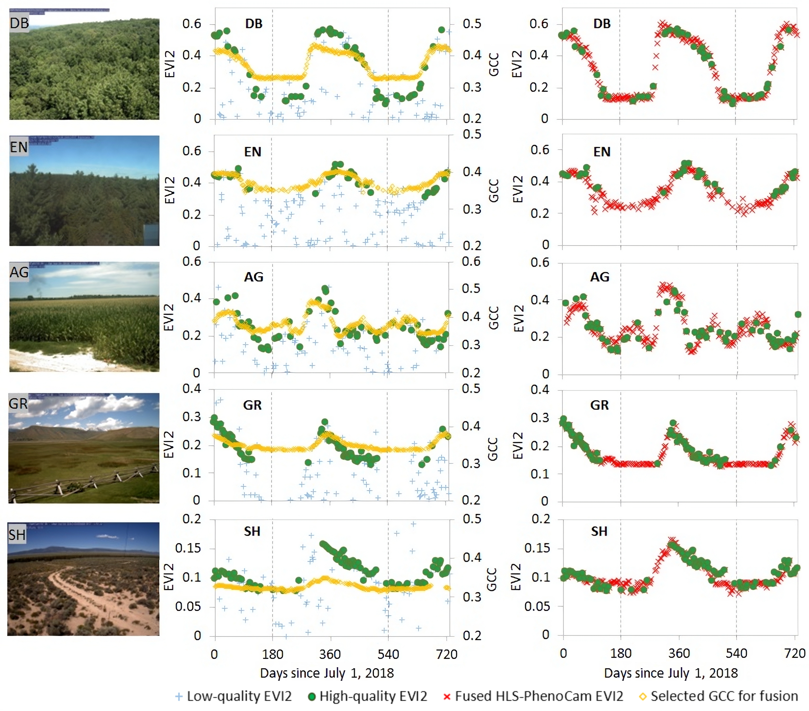
Figure 2. Illustration of fusing HLS EVI2 time series with PhenoCam GCC (Green Chromatic Coordinate) temporal shape to generate 30-m synthetic gap-free HLS-PhenoCam time series for five pixels of deciduous forest (DB), evergreen forest (EN), agriculture (AG), grass (GR), and shrub (SH) nearby PhenoCam sites NEON.D02.SCBI.DP1.00033, howland1, arsgacp1, nationalelkrefuge, nevcanspg1a, respectively. The dates start from July 1, 2018 to July 1, 2020, with the main year 2019 separated by two vertical dash lines.
The HLS-PhenoCam phenometrics were evaluated using the independently-generated near-surface PhenoCam observations. A set of HLS pixels from 78 HLS-PhenoCam regions were spatially matched with the PhenoCam ROIs (Region Of Interest) by visually coordinating the HLS pixel grids with PhenoCam imagery through Google Earth map. The statistical evaluation indicated that the HLS-PhenoCam phenometrics were very close to the near-surface phenology for the years 2019 and 2020 in all four phenological transition dates (greenup onset, maturity onset, senescence onset, and dormancy onset) with R2 ≥ 0.95, MAD ≤ 5 days, RMSE ≤ 8 days, and MSB ≤ 2 days.
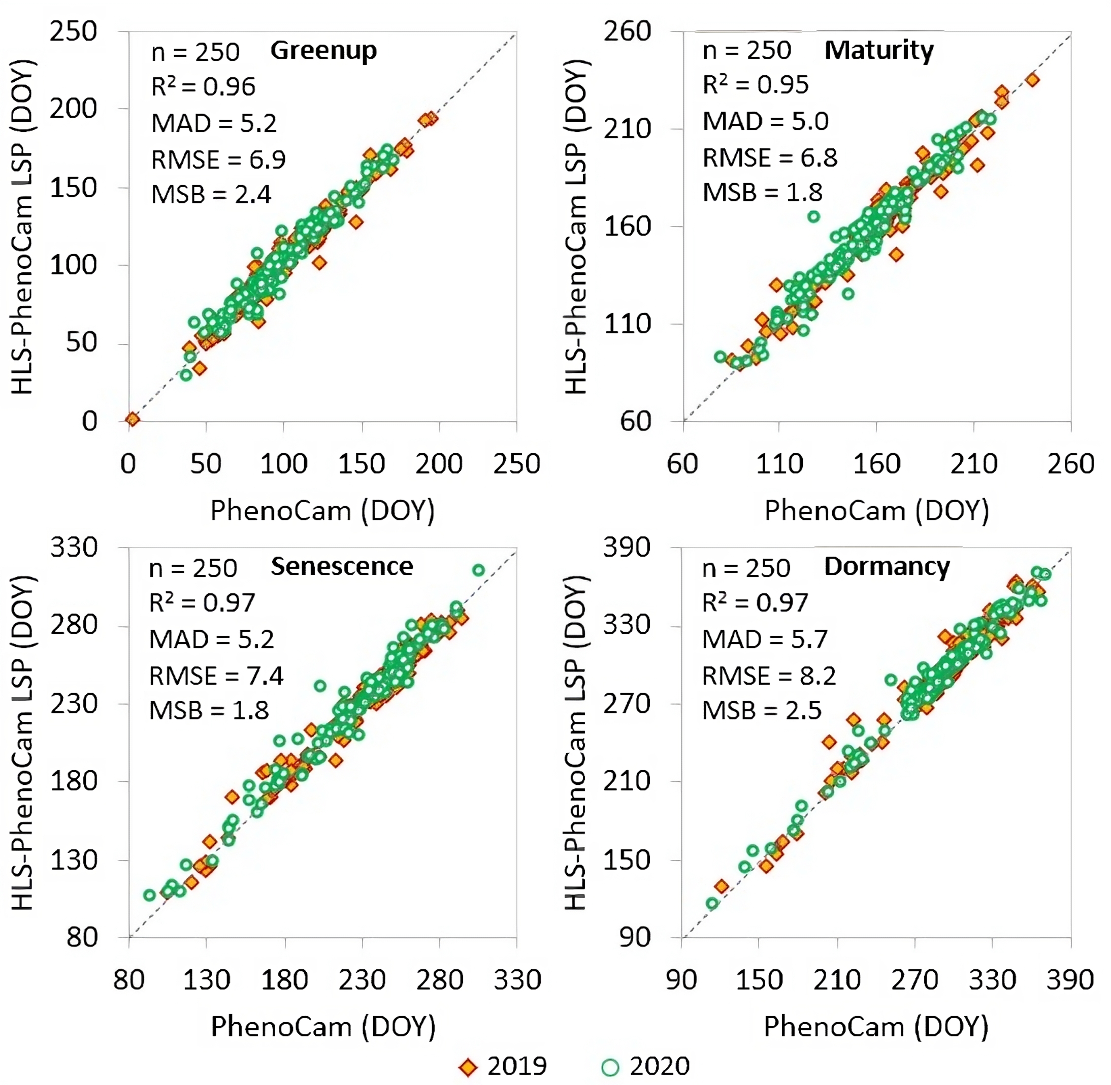
Figure 3. Overall comparison of HLS-PhenoCam phenometrics with near-surface Phenocam observations for four key phenological transition dates (greenup onset, maturity onset, senescence onset, and dormancy onset) in 2019 and 2020. The dashed line indicates the 1:1 agreement.
Data Acquisition, Materials, and Methods
This study used satellite observations (HLS, https://hls.gsfc.nasa.gov/data/v1.4) and near-surface observations (PhenoCam, https://phenocam.nau.edu/) for generating a set of 30-m standardized HLS-PhenoCam LSP datasets. The HLS data are operationally produced from NASA by integrating OLI (Operational Land Imager) aboard the Landsat 8/9 satellites and the MSI (MultiSpectral Instrument) aboard Sentinel-2A/2B satellites. These two measurements enable global observations of the Earth's land surface at a moderate spatial resolution (30 m) and a high temporal resolution (every 2–3 days). Deciduous forests, grasslands, and evergreen forests are the three most common vegetation types captured by PhenoCam cameras, while other vegetation types (e.g., agriculture, shrubs, tundra, and wetland) are less represented. All JPEGs in the archive of 146 PhenoCam sites (refer to Tran et al., 2022) were extracted from the PhenoCam network images between July 1, 2018 and July 1, 2021 from 9 am to 5 pm. The HLS EVI2 data were fused with the most comparable PhenoCam GCC temporal shape selected from the GCC collection using the Spatiotemporal Shape Matching Model (SSMM) to generate the synthetic gap-free HLS-PhenoCam EVI2 time series. The synthetic HLS-PhenoCam EVI2 time series was used to establish the physically-based hybrid piecewise logistic model (HPLM) that was then applied to detect phenological transition dates (phenometrics) of greenup onset, maturity onset, senescence onset, and dormancy onset. Additional details are provided below.
Generation of the 30 m HLS-PhenoCam LSP dataset
The HLS EVI2 (two-band enhanced vegetation index) was selected for detecting land surface phenology (LSP) across 78 regions, each 10 km × 10 km in extent (77 regions in the Contiguous US (CONUS) and one region in Alaska across 30 out of 50 US states) because EVI2 has advantages over other vegetation indices in phenology detections. The QA flags in the HLS product were first used to select only high-quality observations. The 3-day composite of HLS EVI2 time series for a pixel was then generated by selecting or averaging high-quality observations every three days if more than one observation was available. The 3-day HLS EVI2 value was assigned as a fill value (or a gap) when (1) no any high-quality observations exists within the 3-day window, (2) the EVI2 value is greater than 90% of co-located 3-day NDVI (normalized difference vegetation index) value or greater than 110% of any 3-day EVI2 values in the preceding and succeeding one-month period (indication of abiotic noise), or (3) the co-located 3-day NDVI is less than 3-day NDWI (normalized difference water index) (indication of residual contamination from cloud, snow, or land surface moisture).
The PhenoCam GCC (green chromatic coordinate) time series was fully extracted using a newly developed framework instead of using the limited GCC time series available in each site from the PhenoCam dataset version v2.0 (Tran et al., 2022). This framework divides PhenoCam imagery into 10 × 10 grids of equal size in each single PhenoCam site. The resultant grids could reflect considerably different phenological behaviors for either homogeneous or heterogeneous vegetation types captured by the PhenoCam camera in a small area. GCC was calculated for each individual grid on the half-hourly PhenoCam images, which was then aggregated to a 3-day GCC composite by selecting the 90th percentile value. The 3-day GCC composite makes it temporally consistent with the 3-day HLS EVI2 time series. As a result, for every 10 × 10 km2 region selected inside a HLS tile, a diverse collection of grid-based PhenoCam GCC time series was established from all PhenoCam sites located within one and a half HLS tile size. If several 10 × 10 km2 regions are defined within a HLS tile, they use a mutual collection of PhenoCam GCC time series for that HLS tile.
Fusion of HLS and PhenoCam vegetation index time series
The synthetic gap-free HLS-PhenoCam time series was generated by fusing the HLS time series with the PhenoCam time series. The HLS EVI2 time series for a given pixel was compared with each grid-based GCC time series from the PhenoCam GCC collection using the spatiotemporal shape-matching model (SSMM) (equations 1 and 2). The geometric mean functional regression (GMFR) was integrated into the SSMM to calculate mean squared deviation (MSD) and correlation coefficient (R) between raw HLS and predicted HLS values. Ultimately, the PhenoCam GCC time series with the smallest MSD and highest R was selected to fuse with the HLS EVI2 time series. If the HLS EVI2 time series and the best comparable GCC time series were poorly correlated (R ≤ 0.6 and p > 0.02), the fusion was not performed:
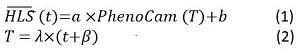 ,
,
where t and T are the time in the number of days, HLS(t), and PhenoCam(T) are predicted HLS EVI2 values at the time t and PhenoCam GCC values at the time T, respectively,
and, a, b, λ, and β are four scaling factors.
In selecting an optimal or comparable GCC time series, λ is set as 0.9 ≤ λ≤ 1.1 with a 0.05 increment, which reflects the ratio of growing season length between HLS and PhenoCam. β is set as-30 ≤ β≤ 30 days with a 3-day increment indicates the seasonal shift between HLS and PhenoCam phenology (Zhang et al., 2020). a and b are the slope and intercept in the linear function in the Eq. (1).
Once the most comparable GCC time series was selected from the collection of PhenoCam GCC time series, its optimal scaling factors a, b, λ, and β were recalled to predict the EVI2 values for all the gaps in the given HLS EVI2 time series using Eq. (1) and (2). Using this approach, a synthetic gap-free HLS-PhenoCam EVI2 time series was generated at a 30-m spatial resolution.
Detection of phenometrics from the synthetic gap-free HLS-PhenoCam EVI2 time series
The Hybrid Piecewise Logistic Model (HPLM) based Land Surface Phenology Detection (LSPD) algorithm was chosen to detect phenological dates from the synthetic HLS-PhenoCam time series (Zhang et al., 2018).
First, the background EVI2 value was calculated by averaging EVI2 values that are smaller than the 10th percentile of the sorted HLS-PhenoCam time series. Second, the HLS-PhenoCam time series was smoothed to further reduce potential noise and irregular variations by using Savitzky-Golay filter and moving average and median methods. Third, the smoothed HLS-PhenoCam time series was divided into greenup and senescence phases by identifying the slope changes using a window of five 3-day values. Fourth, HPLM was applied to reconstruct the greenup and senescence trajectories of vegetation growth cycle (Zhang et al., 2015):
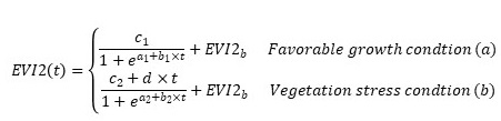 ,
,
where t is time in the day of year (DOY), a is related to the vegetation growth period, b is associated with the rate of plant leaf development, c is the amplitude of EVI2 variation, d is a vegetation stress factor, and EVI2b is the background (dormant season) value.
Finally, four key phenological transition dates or phenometrics (greenup, maturity, senescence, and dormancy onsets) were detected by calculating the local extremes of curvature change rate on the HPLM reconstructed EVI2 time series.
Refer to Tran et al. (2023) for additional information.
Data Access
These data are available through the Oak Ridge National Laboratory (ORNL) Distributed Active Archive Center (DAAC).
Phenology derived from Satellite Data and PhenoCam across CONUS and Alaska, 2019-2020
Contact for Data Center Access Information:
- E-mail: uso@daac.ornl.gov
- Telephone: +1 (865) 241-3952
References
Tran, K.H., X. Zhang, Y. Ye, Y. Shen, S. Gao, Y. Liu, and A. Richardson. 2023. HP-LSP: A reference of land surface phenology from fused Harmonized Landsat and Sentinel-2 with PhenoCam data. Sci Data. (accepted).
Tran, K.H., X. Zhang, A.R. Ketchpaw, J. Wang, Y. Ye, and Y. Shen. 2022. A novel algorithm for the generation of gap-free time series by fusing harmonized Landsat 8 and Sentinel-2 observations with PhenoCam time series for detecting land surface phenology. Remote Sensing of Environment 282:113275. https://doi.org/10.1016/j.rse.2022.113275.
Zhang, X., J. Wang, G.M. Henebry, and F. Gao. 2020. Development and evaluation of a new algorithm for detecting 30 m land surface phenology from VIIRS and HLS time series. ISPRS Journal of Photogrammetry and Remote Sensing 161:37–51. https://doi.org/10.1016/j.isprsjprs.2020.01.012
Zhang, X., L. Liu, Y. Liu, S. Jayavelu, J. Wang, M. Moon, G.M. Henebry, M.A. Friedl, and C.B. Schaaf. 2018. Generation and evaluation of the VIIRS land surface phenology product. Remote Sensing of Environment 216:212–229. https://doi.org/10.1016/j.rse.2018.06.047
Zhang, X. 2015. Reconstruction of a complete global time series of daily vegetation index trajectory from long-term AVHRR data. Remote Sensing of Environment 156:457-472. https://doi.org/10.1016/j.rse.2014.10.012