Documentation Revision Date: 2017-12-21
Data Set Version: V1
Summary
There are eight data files in comma-separated (.csv) format with this dataset. In addition, there are 835 plot photos included as companion files.
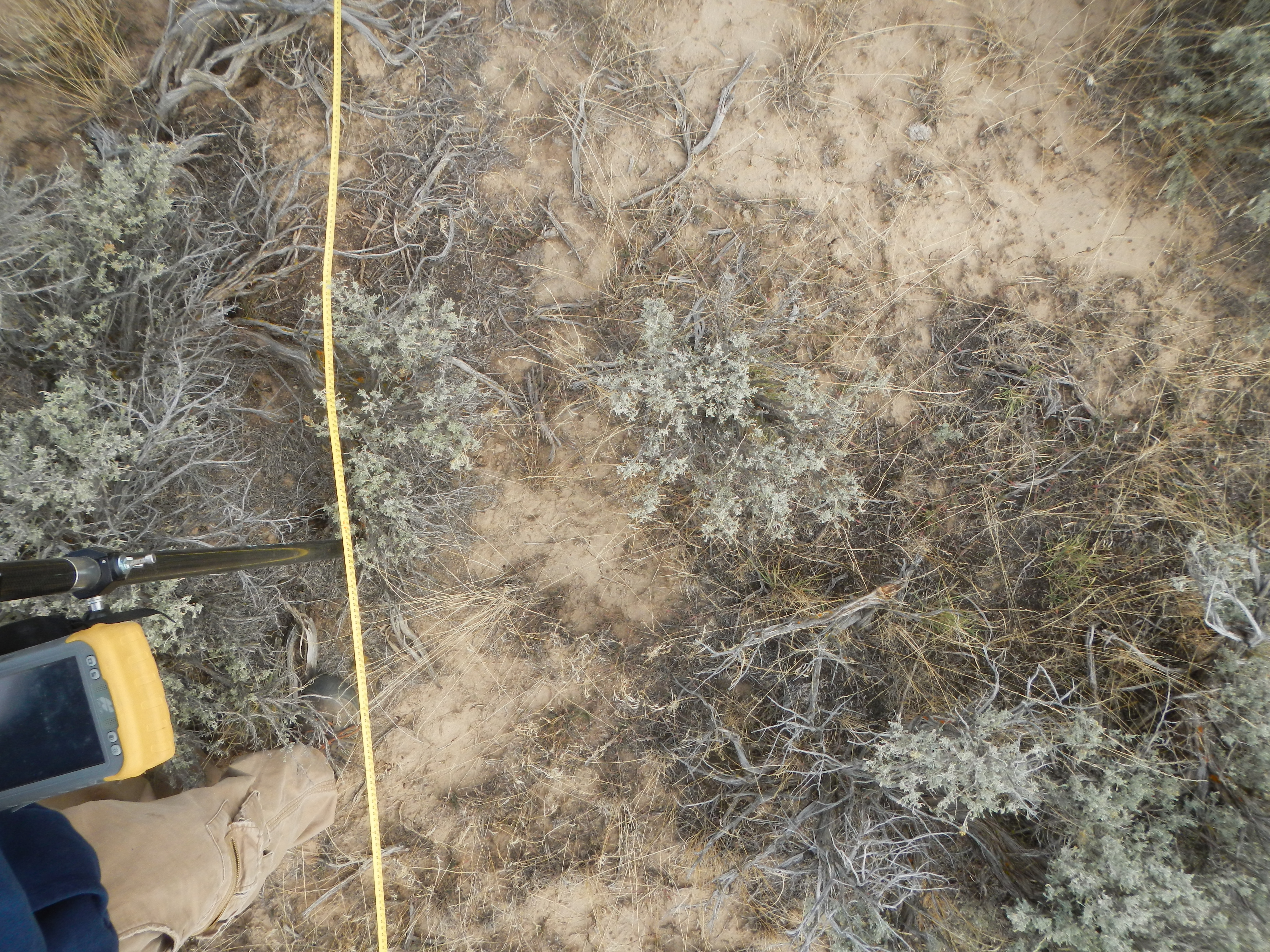
Figure 1. Typical plot photo for ground cover estimates and location of LAI measurements. A rangepole with GPS and a camera boom was positioned at 2-meter intervals along plot transects. This photo is from the Hollister, Sagebrush01 plot, and the Sagebrush01_5_4 sampling point.
Citation
Glenn, N.F., L.P. Spaete, R. Shrestha, A. Li, N. Ilangakoon, J. Mitchell, S.L. Ustin, Y. Qi, H. Dashti, and K. Finan. 2017. Shrubland Species Cover, Biometric, Carbon and Nitrogen Data, Southern Idaho, 2014. ORNL DAAC, Oak Ridge, Tennessee, USA. https://doi.org/10.3334/ORNLDAAC/1503
Table of Contents
- Data Set Overview
- Data Characteristics
- Application and Derivation
- Quality Assessment
- Data Acquisition, Materials, and Methods
- Data Access
- References
Data Set Overview
This dataset provides the results of the characterization of shrubland vegetation at two study areas in southern Idaho, USA: the Reynolds Creek Experimental Watershed (RCEW) and near Hollister. Data were collected in September and October 2014. In each study area, several 10-m x 10-m plots were randomly established that are representative of the local dominant vegetation types. Measurements are reported for both plot and individual shrub attributes. Plot measurements include shrub density and biometric data, percent shrub cover derived from line intercept transects, percent plant species and bare ground cover derived from photo analysis, and average LAI. Measurements for selected individual shrubs include height, width, length, number of stems, and LAI. Leaf samples were collected for determining LAI, specific leaf area (SLA), carbon and nitrogen concentrations, and isotopic nitrogen and carbon.
Related Dataset:
Ilangakoon, N., N. Glenn, and L. Spaete. 2017. LiDAR Data, DEM, and Maximum Vegetation Height Product from Southern Idaho, 2014. ORNL DAAC, Oak Ridge, Tennessee, USA. https://doi.org/10.3334/ORNLDAAC/1532
Acknowledgements:
This research was funded through NASA Terrestrial Ecology grant number NNX14AD81G.
Data Characteristics
Spatial Coverage: Two sites in Southwestern Idaho, USA: Reynolds Creek Experimental Watershed (RCEW) and Hollister, Idaho
Spatial Resolution: Measurements were made on 10 x 10-m plots
Temporal Coverage: 2014-09-16 to 2014-10-17
Temporal Resolution: One-time measurements
Study Area (All latitude and longitude given in decimal degrees)
| Site | Westernmost Longitude | Easternmost Longitude | Northernmost Latitude | Southernmost Latitude |
|---|---|---|---|---|
| Southwestern Idaho, USA: Reynolds Creek Experimental Watershed (RCEW) and Hollister | -116.7973311 | -114.6888979 | 43.20984103 | 42.2990094 |
Data File Information:
There are eight csv data files in this dataset. There are also 835 plot photos included as companion files, provided in Idaho_field_shrub_photos.zip.
Plots were numbered and plot locations are named by the plot number and transects which ran north to south at 1, 3, 5, 7, & 9 meters from the southwest corner, and according to where the samples were taken along each transect at 2, 4, 6, and 8 meters.
Example plot and location: Plot= Bitterbrush01, Plot location= Bitterbrush1_1_2.
Table 1. Data files and descriptions
| File name | Description |
|---|---|
| Idaho_Shrub_Plot_LAI_All.csv | LAI measurements taken at 20 points along the transects in each plot |
| Idaho_Shrub_Plot_LAI_Plot_Mean.csv | Mean LAI for each plot |
| Idaho_Shrub_RTK_GPS_PhotoPlot_LAI_Points.csv | Location of the 20 points along the transects where LAI measurements and plot photos were taken. Includes photo file name for each point. |
| Idaho_Shrub_Photo_Plot_Species_Cover.csv | Species coverage determined from plot photo analysis for each plot |
| Idaho_Shrub_Line_Intercept_Shrub_Cover.csv | Species coverage determined using line intercept method along the transects in each plot |
| Idaho_Shrub_Density.csv | Species, height, and width of all shrubs in each plot |
| Idaho_Shrub_Individuals | Measurements made on individual randomly-chosen dominant species shrubs in the plots |
| Idaho_Shrub_RTK_GPS_Plot_Corners.csv | GPS locations of the plot corners |
Table 2. Idaho_Shrub_Plot_LAI_All.csv
Provides LAI measurements taken at 20 points along the transects in each plot. There are no missing values.
| Variable ID | Units | Description |
|---|---|---|
| study_area | Study area where the data were collected: Reynolds Creek Experimental Watershed (RCEW) and Hollister | |
| year | YYYY | The year the data were collected (all are 2014) |
| plot | The plot name | |
| location | The location along the transect each sample LAI was taken in each 10-m x 10-m plot. Samples were taken along each transect at 2, 4, 6, and 8 meters (locations are illustrated as red dots in Figures 1 and 2) | |
| average_above_par | μmol m-2s-1 | Average above canopy photosynthetically active radiation |
| average_below_par | μmol m-2s-1 | Average below canopy photosynthetically active radiation |
| tau | Tau: the ratio of below canopy PAR measurements to the most recent above canopy PAR value | |
| lai | LAI: the area of leaves per unit area of soil surface | |
| leaf_distribution | The distribution of leaf angles within a canopy (default value =1) | |
| beam_fraction | The ratio of direct beam radiation coming from the sun to radiation coming from all ambient sources (e.g. atmosphere or reflected from other surfaces) | |
| zenith_angle | The angle the sun makes with respect to the zenith, or the point in the sky directly overhead, vertical to where you stand. Calculated using time of day and latitude and longitude | |
| latitude_lai | Degrees | Latitude used for LAI calculation. Do not use for location |
| longitude_lai | Degrees | Longitude used for LAI calculation. Do not use for location |
Table 3. Variables in the file Idaho_Shrub_Plot_LAI_Plot_Mean.csv
Provides the mean LAI from LAI measurements made at the 20 points in the plots (refer to Table 4). There are no missing values.
| Variable ID | Units | Description |
|---|---|---|
| study_area | Study area where the data were collected: Reynolds Creek Experimental Watershed (RCEW) and Hollister | |
| year | YYYY | The year the data were collected (all are 2014) |
| plot | The plot name | |
| average_above_par | μmol m-2s-1 | The average of the average above canopy photosynthetically active radiation for the plot |
| average_below_par | μmol m-2s-1 | The average of the average below canopy photosynthetically active radiation for the plot |
| average_tau | The average Tau for the plot (Tau: the ratio of below canopy PAR measurements to the most recent above canopy PAR value) | |
| average_lai | The average LAI for the plot (LAI: the area of leaves per unit area of soil surface) | |
| leaf_distribution | The average leaf distribution for the plot (The distribution of leaf angles within a canopy (default value =1)) | |
| average_beam_fraction | The average beam fraction for the plot (The ratio of direct beam radiation coming from the sun to radiation coming from all ambient sources (e.g. atmosphere or reflected from other surfaces)) | |
| zenith_angle | The average zenith area for the plot (the angle the sun makes with respect to the zenith, or the point in the sky directly overhead, vertical to where you stand. Calculated using time of day and latitude and longitude) | |
| latitude_lai | Degrees | Latitude used for LAI calculation. Do not use for location |
| longitude_lai | Degrees | Longitude used for LAI calculation. Do not use for location |
Table 4. Variables in the file Idaho_Shrub_RTK_GPS_PhotoPlot_LAI_Points.csv
Provides the RTK GPS points where LAI measurements and photos were taken. There are no missing values.
| Variable ID | Units | Description |
|---|---|---|
| study_area | Study area where the data were collected: Reynolds Creek Experimental Watershed (RCEW) and HollisterD | |
| year | YYYY | The year the data were collected (all are 2014) |
| plot | The plot name | |
| lai_sample_point | The location along the transect in 10 x 10 m plots where each LAI sample was obtained. Transects ran north to south at 1, 3, 5, 7, & 9 meters from the southwest corner. Samples were taken along each transect at 2, 4, 6, and 8 meters | |
| northing | Meters | Northing UTM zone 11N NAD83 datum |
| easting | Meters | Easting UTM zone 11N NAD83 datum |
| longitude | Decimal Degrees | Longitude in WGS84 of photo plot and LAI transect sample |
| latitude | Decimal Degrees | Longitude in WGS84 of photo plot and LAI transect sample |
| elevation | Meters | Elevation in ortho height [NAVD88 (computed using (Geoid2012a)] |
| photo_id | Photo number used for photo plot species cover. Photos are provided in Idaho_field_shrub_photos.zip. |
Table 5. Variables in the file Idaho_Shrub_Photo_Plot_Species_Cover.csv
Provides species coverage at the plots determined from photo analysis. There are no missing values. Symbols for plant species (e.g., CHVI8) are from the USDA, NRCS, PLANTS Database.
| Variable ID | Units | Description |
|---|---|---|
| study_area | Study area where the data were collected: Reynolds Creek Experimental Watershed (RCEW) and Hollister. Photos were collected on 1 m transects at red dots- 2, 4, 6, and 8 meters (Refer to Figure 2) | |
| Year | YYYY | The year the data were collected (all are 2014) |
| Plot | The plot name | |
| cover_ARTRL | % | Percent coverage of plot from 0-100 of sagebrush live |
| cover_ARTRD | % | Percent coverage of plot from 0-100 of sagebrush dead |
| cover_CHVI8L | % | Percent coverage of plot from 0-100 of rabbitbrush live |
| cover_CHVI8D | % | Percent coverage of plot from 0-100 of rabbitbrush dead |
| cover_PUTRL | % | Percent coverage of plot from 0-100 of bitterbrush live |
| cover_PUTRD | % | Percent coverage of plot from 0-100 of bitterbrush dead |
| cover_ UnShL | % | Percent coverage of plot from 0-100 of unknown shrub live |
| cover_UnShD | % | Percent coverage of plot from 0-100 of unknown shrub dead |
| cover_TESP2 | % | Percent coverage of plot from 0-100 of horsebrush |
| cover_ BRTE | % | Percent coverage of plot from 0-100 of cheatgrass |
| cover_POSE | % | Percent coverage of plot from 0-100 of sandberg’s bluegrass |
| cover_ELEL | % | Percent coverage of plot from 0-100 of squirreltail |
| cover_AGDE | % | Percent coverage of plot from 0-100 of desert wheatgrass |
| cover_PSSP | % | Percent coverage of plot from 0-100 of bluebunch wheatgrass |
| cover_UnGr | % | Percent coverage of plot from 0-100 of unknown grass |
| cover_DWD | % | Percent coverage of plot from 0-100 of dead woody debris |
| cover_Forb | % | Percent coverage of plot from 0-100 of forbes |
| cover_Bare | % | Percent coverage of plot from 0-100 of bare soil |
| cover_Rock | % | Percent coverage of plot from 0-100 of rocks or stone |
| cover_Moss | % | Percent coverage of plot from 0-100 of moss |
| cover_Body | % | Percent coverage of plot from 0-100 of person taking picture |
| cover_Litter | % | Percent coverage of plot from 0-100 of organic material not DWD |
| cover_Scat | % | Percent coverage of plot from 0-100 of animal scat |
Table 6. Variables in the file Idaho_Shrub_Line_Intercept_Shrub_Cover.csv
Species coverage determined using line intercept method along the transects. Data not provided are represented as -9999.
| Variable ID | Units | Description |
|---|---|---|
| study_area | Study area where the data were collected: Reynolds Creek Experimental Watershed (RCEW) and Hollister, ID. Coverage was determined along five transects (green lines in Figure 2) | |
| year | YYYY | The year the data were collected (all are 2014) |
| plot | The plot name | |
| sagebrush_dead | % | Percent coverage of plot from 0-1 of sagebrush dead |
| sagebrush_live | % | Percent coverage of plot from 0-1 of sagebrush live |
| bitterbrush_dead | % | Percent coverage of plot from 0-1 of bitterbrush dead |
| bitterbrush_live | % | Percent coverage of plot from 0-1 of bitterbrush live |
| rabbitbrush_dead | % | Percent coverage of plot from 0-1 of rabbitbrush dead |
| rabbitbrush_live | % | Percent coverage of plot from 0-1 of rabbitbrush live |
| snowberry_dead | % | Percent coverage of plot from 0-1 of snowberry dead |
| snowberry_live | % | Percent coverage of plot from 0-1 of snowberry live |
| unknown_dead | % | Percent coverage of plot from 0-1 of unknown shrub dead |
| unknown_live | % | Percent coverage of plot from 0-1 of unknown shrub live |
| Total_Shrub_Cover | % | Percent coverage of plot from 0-1 of all shrubs |
Table 7. Variables in the file Idaho_Shrub_Density.csv
Provides shrub density at the plots. There are no missing values.
| Variable ID | Units | Description |
|---|---|---|
| study_area | Study area where the data were collected: Reynolds Creek Experimental Watershed (RCEW) and Hollister | |
| year | The year the data were collected (all are 2014) | |
| plot | The plot name | |
| plot_transect | The species name_transect number. The transect interspace (blue and white areas in Figure 2) where the shrub height and width data were collected from: 0-1 m, 1-3 m, 3-5 m, 5-7 m, 7-9 m, and 9-10 m | |
| species | The shrub species indicated as live (L) or dead (D). First letter is shrub species (S = sagebrush, B = bitterbrush, R =rabbitbrush, H = horsebrush, Service = Serviceberry (only Live), Juniper = Juniper and U = Unknown Shrub) and last letter is Live or Dead (i.e. SL = Sagebrush Live) | |
| height | cm | The maximum height of the shrub not including flowering or seed stocks |
| major_width | cm | The maximum width of each shrub |
| minor_width | cm | The width perpendicular to the major width |
Table 8. Variables in the file Idaho_Shrub_Individuals.csv
Provides measurements made from six random individual dominant species at the plots. Missing values or those not provided are reported as -9999.
| Variable ID | Units | Description |
|---|---|---|
| study_area | Study area where the data were collected. Reynolds Creek Experimental Watershed (RCEW) and Hollister | |
| year | YYYY | The year the data were collected (all are 2014) |
| plot | The plot name | |
| individual | Measurements taken from six random shrubs (individuals) in the 10 m x 10 m plots. | |
| species | The species of the shrub sampled (Sagebrush, Bitterbrush, Rabbitbrush) | |
| easting | Meters | Easting UTM zone 11N NAD83 datum |
| northing | Meters | Northing UTM zone 11N NAD83 datum |
| longitude | Decimal Degrees | Longitude in WGS84 of individual samples |
| latitude | Decimal Degrees | Latitude in WGS84 of individual samples |
| elevation | meters | Elevation in Ortho Height [NAVD88 (computed using (Geoid2012a)] |
| height | cm | The maximum height of the shrub not including flowering or seed stocks. |
| shrub_max_width | cm | The maximum width of each shrub. |
| width_perpendicular_to_max | cm | The width perpendicular to the major width. |
| average_diameter | cm | Average diameter of stem measured at soil surface. Each stem was measured and then averaged for each individual. |
| number_stems | Number of stems leaving the ground for each individual | |
| lai | LAI: the area of leaves per unit area of soil surface taken for each individual | |
| total_leaf_area | The total leaf area of a subset of leaves taken from each individual shrub. Each subset was selected based on an ocular assessment of leaf size distribution in the field. | |
| wet_weight | mg | The weight of the leaf samples used for total leaf area calculation before drying (obtained from leaf samples of the six shrubs) |
| dry_weight | mg | The weight of the leaf samples used for total leaf area calculation after drying for 48 hrs at 70 degrees C (obtained from leaf samples of the six shrubs) |
| sla | m2/g | Specific Leaf Area (SLA) |
| c | % | Percent Carbon per 100 gram sample (obtained from leaf samples of the six shrubs) |
| d13c | ‰ PDB | d13C (‰ PDB) (obtained from leaf samples of the six shrubs) |
| n | % | Percent nitrogen per 100 gram sample (obtained from leaf samples of the six shrubs) |
| d15n | ‰ AIR | d15N (‰ AIR) (obtained from leaf samples of the six shrubs) |
| Note | Any comments regarding the processing of leaf samples. |
Table 9. Variables in the file Idaho_Shrub_RTK_GPS_Plot_Corners.csv
Provides the RTK GPS of the plot corners. There are no missing values.
| Variable ID | Units | Description |
|---|---|---|
| study_Area | Study area where the data were collected. Reynolds Creek Experimental Watershed (RCEW) and Hollister | |
| year | YYYY | The year the data were collected (all are 2014) |
| plot | The plot name | |
| Plot_Corner | The plot corner (NE, NW, SW, SE) | |
| northing | Meters | Northing UTM zone 11N NAD83 datum |
| easting | Meters | Easting UTM zone 11N NAD83 datum |
| longitude | Decimal Degrees | Longitude in WGS84 of plot corner |
| latitude | Decimal Degrees | Longitude in WGS84 of plot corner |
| elevation | Meters | Elevation in Ortho height [NAVD88 (computed using (Geoid2012a)] |
Application and Derivation
This vegetation field plot data can be used to investigate rangeland ecosystem dynamics. The sampling design is well-suited for multi-scale vegetation analyses with remote sensing.
Quality Assessment
An independent data quality assessment was not performed. Data sheets were reviewed for completeness, including transcription errors.
Data Acquisition, Materials, and Methods
Study Areas
There were two study areas located in southwestern Idaho: Reynolds Creek Experimental Watershed (RCEW) (http://criticalzone.org/reynolds/about/) and Hollister. Forty two 10 x 10-m plots were established in the two study areas. Data were collected between September 16, 2014 and October 17, 2014.
Plot Establishment
Plots were randomly located and corners were marked with half inch rebar. From the initial point, an additional point was located either east or west 10 m and then the final two corners were established to the north of this axis. Real time kinematic (RTK) GPS locations of each corner were collected using a Topcon HiperV RTK GPS. A base GPS was used to collect a static position for at least two hours and a rover GPS unit was used to collect plot locations. The static locations were post processed using OPUS and Magnet Tools was used to apply post processed locations to the GPS locations.
Within each plot, five (5) transects were established at 1, 3, 5, 7, and 9 meters from the southwest corner. Four sampling points were identified (every two meters) along each transect, providing a total of twenty gridded sampling points throughout the plot (see Figure 2).
Plots were named by the dominate plant species and numbered consecutively. Plot sampling points are named by the plot number, transect number (which ran north to south at 1, 3, 5, 7, 9 meters from the southwest corner), and location along transect (at 2, 4, 6, and 8 meters). Example plot and location: Plot= Bitterbrush01, Plot location= Bitterbrush1_1_2.
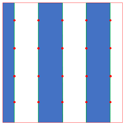
Figure 2. Plots were 10 by 10 meters with transects at 1, 3, 5, 7, and 9 meters. Sampling points were located every 2 meters along each transect.
Measurements at Sampling Points
Photos for ground cover
Plot photos were taken along the transects at the 2, 4, 6, and 8 m sampling points. A rangepole was positioned with a camera boom extending easterly (at each red dot). Locations were recorded with RTK GPS.
Plant species and bare ground percent cover were derived from photo plot analysis.
LAI measurements
LAI measurements were collected at each of the 20 sampling points along the transects using an AccuPAR LP – 80.
Measurements along Transects
Line intercept transects
Species coverage (percent) was derived from line intercept transects. Start and stop locations along 1-m transects were recorded for each shrub species. For example, if there were a sagebrush directly below the transect from 40 cm to 160 cm and a rabbitbrush from 90 cm to 150 cm, the beginning and ending of each would be recorded regardless of overlap.
Species density
Species density was derived by counting all the shrubs between the 0 and 1 m transect line, 1 to 3, 3 to 5, 5 to 7, 7 to 9, and 9 to 10 m lines. The species, major width, and minor width were recorded.
Measurements from individual shrubs
Six individual, random shrubs were chosen for measurements at the plots from the inter-transect areas. Dominant species were selected. At sagebrush plots, a sagebrush was selected, at rabbitbrush plots, a rabbitbrush was selected.
LAI
LAI was also determined for the six individuals. Ten measurements were taken above canopy and 10 below canopy for each shrub. Special care was taken to ensure that light and cloud characteristics remained similar for each measurement.
Specific Leaf Area
Green leaf samples randomly clipped from different portions of each individual random shrub. Samples were scanned with an Epson V600 scanner to determine total leaf area. Samples were then weighed, oven-dried at 70 degrees C for 48 hours, and weighed again to get weight and dry weights respectively. Total leaf area was divided by dry weight to derive SLA.
Foliar carbon and nitrogen
Carbon and Nitrogen were determined for each individual shrub (six random shrubs) using the SLA samples. Samples were ground in a Wiley mill and foliar N and C concentration were measured using a thermo Delta V Plus IRMS (for isotopic nitrogen and carbon) coupled to a Costech ECS 4010 elemental analyzer (Stable Isotope Laboratory, Boise State University).
Data Access
These data are available through the Oak Ridge National Laboratory (ORNL) Distributed Active Archive Center (DAAC).
Shrubland Species Cover, Biometric, Carbon and Nitrogen Data, Southern Idaho, 2014
Contact for Data Center Access Information:
- E-mail: uso@daac.ornl.gov
- Telephone: +1 (865) 241-3952
References
USDA, NRCS. 2017. The PLANTS Database (http://plants.usda.gov, 30 November 2017). National Plant Data Team, Greensboro, NC 27401-4901 USA.