Documentation Revision Date: 2020-08-10
Dataset Version: 1
Summary
There are 2 files in GeoTIFF (*.tif) format.
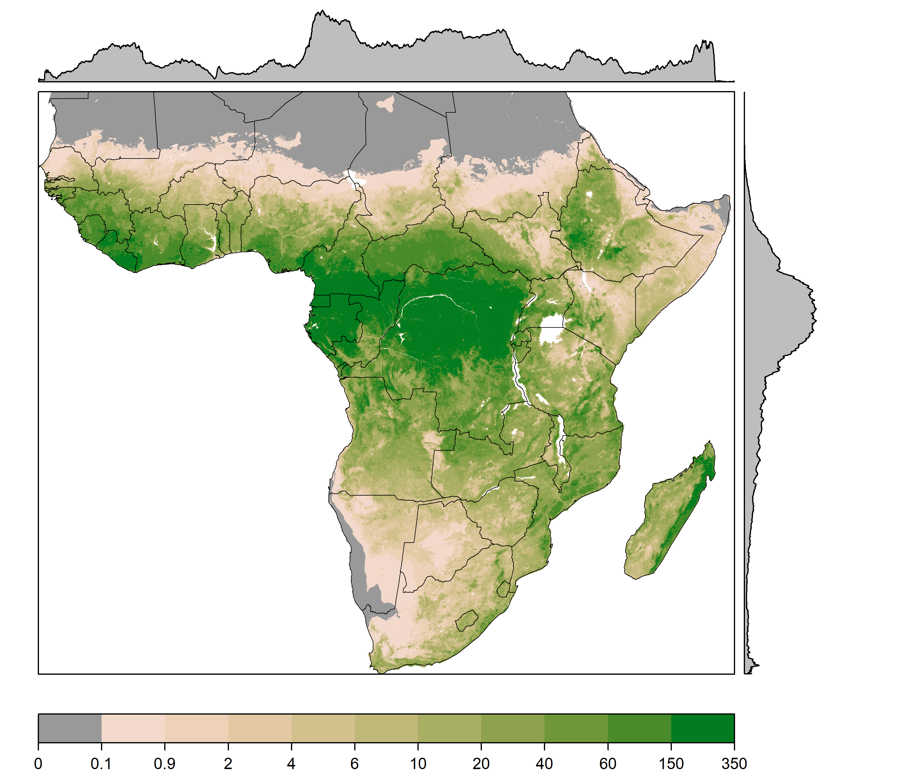
Figure 1. Estimates of woody biomass (tree and shrubs) at 1-km resolution in megagrams per hectare (Mg ha-1). Biomass was estimated from canopy cover, canopy height, and tree allometry. Source: C.W. Ross
Citation
Hanan, N.P., L. Prihodko, C.W. Ross, G. Bucini, and A.T. Tredennick. 2020. Gridded Estimates of Woody Cover and Biomass across Sub-Saharan Africa, 2000-2004. ORNL DAAC, Oak Ridge, Tennessee, USA. https://doi.org/10.3334/ORNLDAAC/1777
Table of Contents
- Dataset Overview
- Data Characteristics
- Application and Derivation
- Quality Assessment
- Data Acquisition, Materials, and Methods
- Data Access
- References
Dataset Overview
This dataset provides maps of woody (tree and shrub) cover and biomass across Sub-Saharan Africa at a resolution of 1 km for the period 2000-2004. Canopy cover observations and remote-sensing data related to woody vegetation were used to predict woody cover across Africa. Predicted woody cover, canopy height, and tree allometry were used to estimate woody biomass for Sub-Saharan Africa. Canopy cover observations were assembled from field measurements and Google Earth imagery collected from 2000-2004. Remote-sensing data related to the structural attributes of woody vegetation were derived from MODIS optical data and Q-SCAT (Quick Scatterometer) microwave measurements. Canopy height estimates were derived from spaceborne lidar and tree allometry equations were retrieved from GlobAllomeTree.
Acknowledgments:
This work was supported by the NASA Carbon Cycle Science grant NNX17AI49G.
Data Characteristics
Spatial Coverage: Sub-Saharan Africa
Spatial Resolution: 1 km
Temporal Coverage: 2000-01-01 to 2004-12-31
Temporal Resolution: One time, five-year average
Study Area: Latitude and longitude are given in decimal degrees.
|
Site |
Westernmost Longitude |
Easternmost Longitude |
Northernmost Latitude |
Southernmost Latitude |
|---|---|---|---|---|
| Sub-Saharan Africa | -20.60774 | 61.52528 | 22.00811 | -34.81449 |
Data File Information
This dataset includes 2 files in GeoTIFF (*.tif) format.
Table 1. File names and descriptions.
|
File Name |
Units |
Description |
|---|---|---|
| woody_biomass.tif | Mg ha-1 | an estimate of woody biomass in megagrams per hectare |
| woody_cover.tif | percent | the proportion of a cell predicted to have woody cover |
Data File Details
Missing values are represented by -3400 in woody_biomass.tif and 255 in woody_cover.tif. Each file contains 6289 rows and 7515 columns. The projection used is "World_Sinusoidal", EPSG:54008.
Application and Derivation
These data were produced to support studies investigating the role of woody vegetation in ecology, carbon cycle, biogeochemistry, and land surface-atmosphere interactions of the African continent.
Quality Assessment
Canopy Cover Evaluation & Comparison with Existing Products
When estimating woody cover from Google Earth imagery, the ambiguous crown identification was recorded to estimate the error in measurements (± 3.7% woody cover).
Model training was performed on 775 field-based canopy cover measurements, and model evaluation was performed by comparing predicted cover against a held-out validation set, which consisted of 259 field-based measurements. Model evaluation with the independent validation set indicated that the model explained 67% of the variation in woody canopy cover, corresponding to a root mean square error (RMSE) of 10.8%.
Canopy Height Evaluation
Model evaluation indicated that local calibration error was 4.1 m (R2 = 0.84) and wall-to-wall model RMSE was 6.6 m (R2 = 0.64). See Simard et al. (2011) for a thorough description of model development and error assessment.
Woody Biomass Evaluation
Woody biomass estimates were compared with existing woody biomass estimates for Africa at the national level (Table 2). Total aboveground biomass for each country was converted to carbon using a conversion factor of 0.5. While estimates of carbon stocks were in general agreement with other satellite-based estimates, the values provided in this dataset are lower on average.
Table 2. Comparison between woody biomass carbon stock estimates (Mt C) available from different sources.
| Country | Land Area (km2) | This Study | Bouvet et al. (2018) | Saatchi et al. (2011) | Baccini et al. (2012) | Avitabile et al. (2016) |
|---|---|---|---|---|---|---|
| Angola | 1275231 | 1673 | 2786 | 3322 | 4742 | 2041 |
| Benin | 116837 | 123 | 180 | 162 | 212 | 33 |
| Congo | 341223 | 2768 | 3358 | 3209 | 3333 | 4098 |
| DemRepCongo | 2332349 | 16581 | 17746 | 18195 | 21867 | 19966 |
| Burundi | 26968 | 60 | 51 | 73 | 74 | 22 |
| Cameroon | 467694 | 3305 | 3393 | 3700 | 3650 | 4322 |
| Chad | 1315774 | 142 | 509 | NA | NA | NA |
| CentAfrRep | 623022 | 2569 | 2583 | 2428 | 3404 | 1762 |
| Djibouti | 22104 | 1 | 30 | 7 | 5 | 8 |
| Equatorial Guinea | 26964 | 287 | 316 | 363 | 253 | 454 |
| Eritrea | 123952 | 36 | 115 | 53 | 40 | 34 |
| Ethiopia | 1142267 | 1446 | 2260 | 2003 | 1812 | 822 |
| Gambia | 10970 | 5 | 32 | 9 | 14 | 2 |
| Gabon | 264143 | 2719 | 3377 | 3448 | 2624 | 4453 |
| Ghana | 240131 | 573 | 522 | 601 | 680 | 325 |
| Guinea | 248210 | 680 | 1262 | 807 | 855 | 234 |
| Cote d'Ivoire | 323831 | 1131 | 944 | 1105 | 1282 | 584 |
| Kenya | 580858 | 387 | 977 | 804 | 519 | 273 |
| Liberia | 96334 | 766 | 878 | 1003 | 904 | 1172 |
| Libya | 1807520 | 0 | 41 | NA | NA | NA |
| Madagascar | 625517 | 1333 | 1941 | 1906 | NA | 1202 |
| Mali | 1307669 | 182 | 417 | NA | NA | NA |
| Mauritania | 1106930 | 7 | 40 | NA | NA | NA |
| Mozambique | 822837 | 1246 | 1964 | 2302 | NA | 889 |
| Malawi | 120965 | 115 | 153 | 218 | 269 | 76 |
| Niger | 1237580 | 15 | 85 | NA | NA | NA |
| Nigeria | 919182 | 1367 | 1855 | 1572 | 1655 | 675 |
| Guinea-Bissau | 34474 | 71 | 94 | 88 | 105 | 25 |
| Rwanda | 25236 | 73 | 61 | 72 | 73 | 31 |
| South Africa | 1388689 | 466 | 829 | 1706 | NA | 493 |
| Lesotho | 34843 | 23 | 13 | 43 | NA | 15 |
| Botswana | 622179 | 79 | 337 | 329 | NA | 131 |
| Senegal | 202015 | 76 | 195 | 192 | 181 | 48 |
| Sierra Leone | 73252 | 313 | 276 | 346 | 407 | 215 |
| Somalia | 635865 | 118 | 989 | 397 | 237 | 248 |
| Sudan | 2580717 | 720 | 1439 | 979 | 1701 | 231 |
| Togo | 57521 | 94 | 76 | 108 | 125 | 26 |
| Tanzania | 946097 | 1172 | 1800 | 2010 | 2710 | 800 |
| Uganda | 241018 | 424 | 421 | 495 | 591 | 217 |
| Burkina Faso | 280518 | 89 | 251 | 151 | 146 | 44 |
| Namibia | 887156 | 84 | 622 | 281 | NA | 168 |
| Swaziland | 19235 | 17 | 31 | 47 | NA | 15 |
| Zambia | 770823 | 906 | 1642 | 2086 | 2816 | 1012 |
| Zimbabwe | 411819 | 226 | 607 | 764 | 670 | 154 |
| Total | 26738519 | 44473 | 57498 | 57384 | 57956 | 47320 |
Data Acquisition, Materials, and Methods
Canopy Cover Observations
A dataset of 1034 canopy cover estimates for trees and shrubs was assembled from field-based measurements across Africa and supplemented in under-sampled regions (desert margins and moist tropical forests) by visual analysis of high-resolution imagery (Fig. 2). Most of the field measurements were compiled in 2000-2004 in African savannas (Sankaran et al., 2005). Additional field measurements were provided from three field surveys: 69 points in the Kruger National Park, South Africa (Bucini et al. 2010), 12 points in Uganda (Mitchard et al. 2009), and 49 points in Zambia. Plots falling within the same 1 km pixel were averaged, resulting in 803 field-based data points.
Google Earth (GE; http://earth.google.com) imagery collected between 2000 and 2005 was used to estimate woody cover at 173 locations, including forest and seasonal woodlands, deserts, and agricultural areas. A 1-km by 1-km geo-rectified grid was overlaid on the GE images divided into 16 cells (250 m2), and an 8 x 8 point sub-grid was deployed within each cell. The fractional cover of a cell was estimated by the presence and absence of woody plant crowns under the digital point samples.
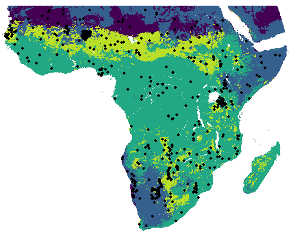
Figure 2. Distribution of sites (N = 1,034) contributing woody cover data including field data (Sankaran et al, 2005) and estimates from high-resolution satellite imagery. (Source C. W. Ross)
Canopy Cover Covariates
Remote-sensing data were compiled from both optical and microwave sensors operating from 2000-2004 and were limited to metrics linked to structural attributes of woody vegetation. MODIS composite reflectance was used to minimize cloud and atmospheric contamination, resulting in monthly average reflectance data at 1-km resolution. Monthly average red (R) and near-infrared (NIR) reflectance were used to calculate monthly average normalized difference vegetation index (NDVI=(NIR-R)/(NIR+R)), mean annual NDVI (“ND_mean”) and the difference between growing season and dry-season mean NDVI (“ND_diff”), which provides information related to phenological variability.
Imagery from Q-SCAT (Quick Scatterometer) available in three-day composites at 2.25-km resolution for years 2000-2004 was processed into average monthly composite and resampled at 1-km resolution. Two metrics were calculated from the data: the annual averaged backscatter (“QS_mean”) and the standard deviation (“QS_sd”) in the HH polarization.
The combination of optical data from MODIS and microwave backscatter from Q-SCAT offered two optical remote sensing metrics (ND_mean, ND_diff) and two microwave metrics (QS_mean, QS_sd) covering Sub-Saharan Africa and projected to a common 1 km spatial resolution sinusoidal grid projection.
Predicting Woody Cover
Fractional woody cover (y) located within pixel i was modeled as conditionally binomial
y_i∼Binomial(p_i,100) (1)
logit(p_i) = α+ x_iβ (2)
where p_i is the probability of success (expected proportional woody cover) out of 100 trials for pixel i, x is the vector of remote-sensing covariates for pixel i, α is the intercept, and β is the vector of effect terms for the remote-sensing covariates. Remote-sensing covariates were standardized [(x_i-x)/σ(x)] to improve convergence during the model fitting stage and to allow for an easier prior specification.
Each model was fit using a subset of the complete dataset (75%; N = 775) and then using the remaining held-out data (25%; N = 259) to calculate the out-of-sample predicted fit as the log predictive density (Eq. 3):
lpd = log∫ [y_val |θ][θ]|y_train]dθ (3)
where lpd is a local and proper scoring function for Bayesian validation (Gelman et al., 2014), and is approximated from Markov chain Monte Carlo (Eq. 4), θ is the set of all unknown parameters to be estimated by the model.
lpd = log[y_val | y_train] ≈log∑_(k=1)^K y_val | y_train]/K (4)
where k is a single iteration and K is the total number of MCMC iterations (Hooten and Hobbs, 2015). The model with the highest lpd was considered to be the optimal predictive model and was used to estimate parameters for spatial mapping of woody percent cover.
The three optimally-predictive model sets provide ensemble predictions of tree cover for every terrestrial location in sub-Saharan Africa using different combinations of variables derived from MODIS optical data and Qscatt microwave measurements. The final multi-model ensemble prediction approach is summarized in Table 3.
The posterior prediction scores were calculated from three MCMC chains comprised of 1000 iterations each after discarding an initial 1000 iterations as burn-in. After selecting the optimally predictive model based on lpd, that model was fit using only the training data to obtain posterior distributions of all model parameters from three MCMC chains comprised of 1000 iterations each after discarding an initial 1000 iterations as burn-in.
Table 3. Multi-model ensemble prediction approach for different mean annual rainfall (MAP) climate zones of Sub-Saharan Africa.
| Bioclimate Zone |
MAP Range (mm/year) |
Ensemble Estimation Approach | Index |
|---|---|---|---|
| Desert | MAP < 100 | TC = 0% | 0 |
| Arid savanna | 100 < MAP < 600 | 3-model median (median[1,2,3]) | 1 |
| Semi-arid savanna | 600 < MAP < 1000 | 3-model average (mean[1,2,3]) | 2 |
| Mesic savanna & forest | 1000<MAP | 2-model average (mean[1,3]) | 3 |
| Sankaran constraint on maximum TC predictions | 100 < MAP < 1000 | Use Sankaran potential TC if < multi-model TC prediction | 4 |
Canopy Height
The source of canopy height estimates was Simard et al. (2011). They derived global canopy height at 1-km resolution from 2005 Geoscience Laser Altimeter System (GLAS) aboard ICESat (Ice, Cloud, and land Elevation Satellite) and covariates. Canopy height was integrated into the Spatial Data Access Tool (ORNL DAAC, 2017) for reprojection and download. Gridded canopy height data are available for download at https://webmap.ornl.gov/ogc/dataset.jsp?dg_id=10023_1.
When canopy height was not available where canopy cover was greater than 0%, linear regression was used to model and predict canopy height as a function of long-term mean-annual precipitation (Fick and Hijmans, 2017). Unavailable canopy height values were primarily confined to semi-arid and arid regions with low mean annual precipitation, where trees and shrubs tend to have relatively low canopy cover and short stature due to water constraints. Canopy height was then re-projected to the same coordinate system and resolution as the canopy cover data.
Allometric Relationships to Calculate Biomass
Global tree allometry data were retrieved from GlobAllomeTree (www.globallometree.org) and subset to calculate the relationship between biomass, tree height, and canopy cover in Africa:
B/C = exp¡(-1.19909+ln(H)*1.27841 (5)
where B/C is woody biomass (kg) per square meter of canopy cover, and H is height.
Continental-scale biomass estimates were then obtained:
Biomass = (wc/100)*10,000*B/C (6)
where Biomass is tree and shrub biomass (Mg ha-1), wc is predicted woody cover (%), and B/C is obtained from Eq. 5.
Data Access
These data are available through the Oak Ridge National Laboratory (ORNL) Distributed Active Archive Center (DAAC).
Gridded Estimates of Woody Cover and Biomass across Sub-Saharan Africa, 2000-2004
Contact for Data Center Access Information:
- E-mail: uso@daac.ornl.gov
- Telephone: +1 (865) 241-3952
References
Avitabile, V., Herold, M., Heuvelink, G.B.M., Lewis, S.L., Phillips, O.L., Asner, G.P., Armston, J., Ashton, P.S., Banin, L., Bayol, N., et al. (2016). An integrated pan-tropical biomass map using multiple reference datasets. Glob. Change Biol. 22, 1406–1420. https://doi.org/10.1111/gcb.13139
Baccini, A., Goetz, S.J., Walker, W.S., Laporte, N.T., Sun, M., Sulla-Menashe, D., Hackler, J., Beck, P.S.A., Dubayah, R., Friedl, M.A., et al. (2012). Estimated carbon dioxide emissions from tropical deforestation improved by carbon-density maps. Nat. Clim. Change 2, 182–185. https://doi.org/10.1038/nclimate1354
Bouvet, A., Mermoz, S., Le Toan, T., Villard, L., Mathieu, R., Naidoo, L., and Asner, G.P. (2018). An above-ground biomass map of African savannahs and woodlands at 25m resolution derived from ALOS PALSAR. Remote Sens. Environ. 206, 156–173. https://doi.org/10.1016/j.rse.2017.12.030
Bucini, G., Hanan, N.P., Boone, R.B., Smit, I.P.J., Saatchi, S.S., Lefsky, M.A., Asner, G.P., Hanan, N.P., Boone, R.B., Smit, I.P.J., et al. (2010). Woody Fractional Cover in Kruger National Park, South Africa: Remote Sensing–Based Maps and Ecological Insights. https://doi.org/10.1201/b10275
Fick, S.E., and Hijmans, R.J. (2017). WorldClim 2: new 1-km spatial resolution climate surfaces for global land areas. Int. J. Climatol. 37, 4302–4315. https://doi.org/10.1002/joc.5086
Gelman, A., Hwang, J., and Vehtari, A. (2014). Understanding predictive information criteria for Bayesian models. Stat. Comput. 24, 997–1016. https://doi.org/10.1007/s11222-013-9416-2
Hooten, M.B., and Hobbs, N.T. (2015). A guide to Bayesian model selection for ecologists. Ecol. Monogr. 85, 3–28. https://doi.org/10.1890/14-0661.1
Mitchard, E.T.A., Saatchi, S.S., Woodhouse, I.H., Nangendo, G., Ribeiro, N.S., Williams, M., Ryan, C.M., Lewis, S.L., Feldpausch, T.R., and Meir, P. (2009). Using satellite radar backscatter to predict above-ground woody biomass: A consistent relationship across four different African landscapes. Geophys. Res. Lett. 36. https://doi.org/10.1029/2009GL040692
Saatchi, S.S., Harris, N.L., Brown, S., Lefsky, M., Mitchard, E.T.A., Salas, W., Zutta, B.R., Buermann, W., Lewis, S.L., Hagen, S., et al. (2011). Benchmark map of forest carbon stocks in tropical regions across three continents. Proc. Natl. Acad. Sci. 108, 9899–9904. https://doi.org/10.1073/pnas.1019576108
Sankaran, M., Hanan, N.P., Scholes, R.J., Ratnam, J., Augustine, D.J., Cade, B.S., Gignoux, J., Higgins, S.I., Roux, X.L., Ludwig, F., et al. (2005). Determinants of woody cover in African savannas. Nature 438, 846. https://doi.org/10.1038/nature04070
Simard, M., N. Pinto, J. B. Fisher, and A. Baccini (2011), Mapping forest canopy height globally with spaceborne lidar, J. Geophys. Res., 116, G04021, https://doi.org/10.1029/2011JG001708.