Documentation Revision Date: 2025-07-07
Dataset Version: 1
Summary
This dataset includes a total of 116 datafiles: 79 cloud-optimized GeoTIFFs (*.tif), 13 ENVI (paired *.bin and *.hdr) files, 21 comma separated values (*.csv) files, two shapefiles (*.shp), and one zip file holding three files of R code.
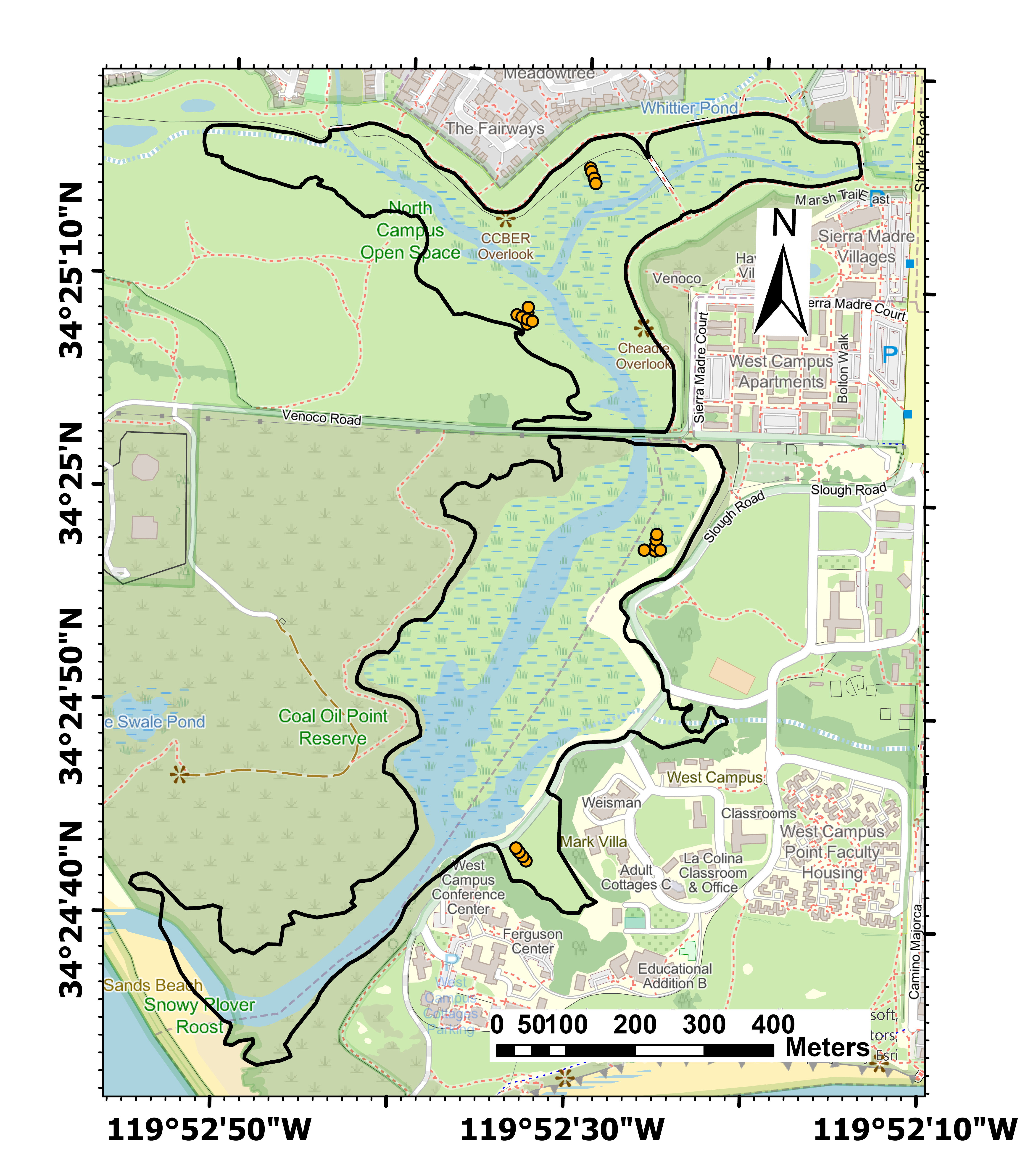
Figure 1. Soil and spectra sampling locations (orange circles) within Devereux Slough, California, U.S.
Citation
Silva, G.D., M. Arndt, B. Lee, C. Liu, E. Phillips, R. Song, N. Taylor, and K.B. Byrd. 2025. SHIFT: Wetland Spectra, Salinity, and Fractional Cover, Devereux Slough, CA, 2022. ORNL DAAC, Oak Ridge, Tennessee, USA. https://doi.org/10.3334/ORNLDAAC/2436
Table of Contents
- Dataset Overview
- Data Characteristics
- Application and Derivation
- Quality Assessment
- Data Acquisition, Materials, and Methods
- Data Access
- References
Dataset Overview
This dataset includes field data, analysis code, and imagery collected and generated during the 2022 NASA Surface Biology Geology (SBG) High Frequency Time series (SHIFT) campaign within Devereux Slough estuary in Santa Barbara County, California, USA. This project collected field data contemporaneously with weekly flights of the NASA's Airborne Visible-Infrared Imaging Spectrometer-Next Generation (AVIRIS-NG) facility instrument over the study areas. Soil samples were collected in North Campus Open Space and Coal Oil Point Reserve between 2022-02-24 to 2022-09-16 and analyzed for salinity (electric conductivity). Soil samples were paired with corresponding AVIRIS-NG flights, and AVIRIS-NG Level 2A Unrectified Reflectance data were used to derive fractional cover and vegetation and soil indices across the study area (Figure 1). Multiple endmember spectral mixture analysis (MESMA) was used to estimate fractional cover for four cover classes. Additionally, canopy response stress index, modified anthocyanin reflectance index, normalized difference vegetation index, and vegetation soil salinity index were derived.
Project: SHIFT
The Surface Biology and Geology (SBG) High Frequency Time Series (SHIFT) was an airborne and field campaign during February to May, 2022, with a follow up activity for one week in September, in support of NASA's SBG mission. Its study area included a 640-square-mile (1,656-square-kilometer) area in Santa Barbara County and the coastal Pacific waters. The primary goal of the SHIFT campaign was to collect a repeated dense time series of airborne Visible to ShortWave Infrared (VSWIR) airborne imaging spectroscopy data with coincident field measurements in both inland terrestrial and coastal aquatic areas, supported in part by a broad team of research collaborators at academic institutions. The SHIFT campaign leveraged NASA's Airborne Visible-Infrared Imaging Spectrometer-Next Generation (AVIRIS-NG) facility instrument to collect approximately weekly VSWIR imagery across the study area. The SHIFT campaign 1) enables the NASA SBG team to conduct traceability analyses related to the science value of VSWIR revisit without relying on multispectral proxies, 2) enables testing algorithms for consistent performance over seasonal time scales and end-to-end workflows including community distribution, and 3) provides early adoption test cases to SHIFT application users and incubate relationships with basic and applied science partners at the University of California Santa Barbara Sedgwick Reserve and The Nature Conservancy's Jack and Laura Dangermond Preserve.
Related Publication:
Silva, G.D., D.A. Roberts, K.B. Byrd, K.D. Chadwick, I.J. Walker, and J.Y. King. 2025. Using imaging spectroscopy and elevation in machine learning to estimate soil salinity in intermittently tidal wetlands. Ecosphere (in press).
Related Datasets
Brodrick, P., R. Pavlick, M. Bernas, J.W. Chapman, R. Eckert, M. Helmlinger, M. Hess-Flores, L.M. Rios, F.D. Schneider, M.M. Smyth, M. Eastwood, R.O. Green, D.R. Thompson, K.D. Chadwick, and D.S. Schimel. 2023. SHIFT: AVIRIS-NG L2A Unrectified Reflectance. ORNL DAAC, Oak Ridge, Tennessee, USA. https://doi.org/10.3334/ORNLDAAC/2183
Acknowledgments
This research was supported by NASA's Surface Biology and Geology (SBG) Mission (Pre-Phase A).
Data Characteristics
Spatial Coverage: Devereux Slough, Santa Barbara County, CA, USA
Spatial Resolution: 5 m for gridded data; point resolution for vector data; soil samples collected from 0 - 15 cm depth
Temporal Coverage:
Precipitation data: 2007-05-26 to 2024-05-30
Field measurements: 2022-02-25 to 2022-09-11
Spectral measurements: 2022-02-24 to 2022-05-29
Temporal Resolution: 15 minutes for precipitation; weekly for field and spectral measurements.
Site Boundaries: Latitude and longitude are given in decimal degrees.
| Site | Westernmost Longitude | Easternmost Longitude | Northernmost Latitude | Southernmost Latitude |
|---|---|---|---|---|
| Devereux Slough, Santa Barbara County, CA, USA | -119.8943 | -119.8613 | 34.4311 | 34.4040 |
Data File Information
This dataset includes a total of 115 datafiles: 79 cloud-optimized GeoTIFFs (*.tif), 13 ENVI (paired *.bin and *.hdr) files, 21 comma separated values (*.csv) files, two shapefiles (*.shp), and one zip file holding three files of R code.
There are three categories of files: spectral data, field data, and geospatial data:
Spectral Data
Spectral data are contained in 78 cloud-optimized GeoTIFFs, 13 ENVI, and 19 comma separated values (*.csv) files:
- AVIRIS-NG Level 2A Unrectified Reflectance: 13 ENVI files (paired *.bin and *.hdr files) containing AVIRIS-NG Level 2A spectra (Brodrick et al. 2023) data clipped to the study area.
Files are named: rfl_<YYYYMMDD>.<ext>, where <YYYYMMDD> is the AVIRIS-NG flight date and <ext> is the file extension ("bin" indicates ENVI binary; "hdr" indicates ENVI header file).- Coordinate system: projected in UTM zone 11 N, WGS 84, (EPSG 32611)
- Spatial resolution: 4.8 m
- Number of bands: 425 (one per wavelength)
- Canopy Response Stress Index (CRSI): 13 GeoTIFF files, one for each AVRIS-NG flight date.
Files are named: CRSI_<YYYYMMDD>.tif, where <YYYYMMDD> is the AVIRIS-NG flight date. - Fractional Cover: 13 GeoTIFF files, one for each AVRIS-NG flight date, showing fractional cover at 5-m resolution.
Files are named: fractional_cover_rfl_<YYYYMMDD>.tif. All fractions range from 0 to 1.- Number of bands: 8
- Band_1 = BARE SOIL_fraction: fraction of pixel that is bare soil.
- Band_2 = GREEN VEG_fraction: fraction of pixel that is green vegetation.
- Band_3 = NPV_fraction: fraction of pixel that is non-photosynthetic vegetation.
- Band_4 = WATER_fraction: fraction of pixel that is water.
- Band_5 = shade_fraction: fraction of pixel that is shaded.
- Band_6 = RMSE: Root-mean square error between reference endmember spectra and individual pixel spectrum
- Band_7 = Complexity: number of endmember classes used to unmix the spectrum (4 indicating 3 fractions + shade for the pixel)
- Band_8 = model#: model identification number, the exact combination of endmembers that were used to unmix each pixel. Please see the associated fractional cover model output for additional details.
- Number of bands: 8
- Fractional Cover Model Outputs: 13 comma separated values files, one for each AVRIS-NG flight date, containing the multiple endmember spectral mixture analysis (MESMA) outputs from the fractional cover model.
Files are named: fractional_cover_rfl_<YYYYMMDD>_models.csv.- No data value: -9999 for numeric fields and ‘N/A’ for text fields
- Modified Anthocyanin Reflectance Index (mARI): 13 GeoTIFF files, one for each AVRIS-NG flight date.
Files are named: mARI_avg_<YYYYMMDD>.tif. - Normalized Difference Vegetation Index (NDVI): 13 GeoTIFF files, one for each AVRIS-NG flight date.
Files are named: NDVI_<YYYYMMDD>.tif. - Point Spectra: Six comma separated values files, one for each field sampling site (3) across two dates. Files contain the wavelengths and reflectance values from AVIRIS-NG Level 2 spectra (Brodrick et al. 2023) for points along individual transects at sampling sites. See Table 2 for the location information for each point.
Files are named: spectra_<Site>_<Dir>_<YYYYMMDD>.csv, where <Site> is Coal Oil Point Reserve #2 (‘COPR_2’) or North Campus Open Space #1 or #2 (‘NCOS_1’; ‘NCOS_2’), <Dir> is the transect direction is north-south (‘ns’) or east-west (‘ew’), and <YYYYMMDD> is AVIRIS-NG flight date. - Shade-normalized Fractional Cover: 13 GeoTIFF files, one for each AVRIS-NG flight date.
Files are named: shade_norm_rfl_<YYYYMMDD>.tif.- Number of bands: 8
- Band_1 = BARE SOIL_fraction: fraction of pixel that is bare soil.
- Band_2 = GREEN VEG_fraction: fraction of pixel that is green vegetation.
- Band_3 = NPV_fraction: fraction of pixel that is non-photosynthetic vegetation.
- Band_4 = WATER_fraction: fraction of pixel that is water.
- Band_5 = shade_fraction: fraction of pixel that is shaded.
- Band_6 = RMSE: Root-mean square error between reference endmember spectra and individual pixel spectrum
- Band_7 = Complexity: number of endmember classes used to unmix the spectrum (4 indicating 3 fractions + shade for the pixel)
- Band_8 = model#: model identification number, the exact combination of endmembers that were used to unmix each pixel. Please see the associated fractional cover model output for additional details.
- Number of bands: 8
- Vegetation Soil Salinity Index (VSSI): 13 GeoTIFF files, one for each AVRIS-NG flight date.
Files are named: VSSI_<YYYYMMDD>.tif.
Spectral Data GeoTIFF characteristics
- Coordinate system: UTM zone 11N, WGS 84 datum (EPSG 32611)
- Spatial resolution: 5 m
- Map units: meters
- No data value: -9999
- Number bands: 1 for most; fractional_cover_rfl_<YYYYMMDD>.tif and shade_norm_rfl_<YYYYMMDD>.tif have 8 bands.
Table 1: Data dictionary for fractional cover model outputs (fractional_cover_rfl_<YYYYMMDD>_models.csv)
| Variable | Units | Description |
|---|---|---|
| Model_number | - | Model identification number |
| EM_number | - | The number of endmember classes used in the model |
| Model | - | Which specific endmember classes used |
| BARE_SOIL | - | Name of bare soil endmember spectrum (if used) |
| GREEN_VEG | - | Name of green vegetation endmember spectrum (if used) |
| NPV | - | Name of non-photosynthetic vegetation endmember spectrum (if used) |
| WATER | - | Name of water endmember spectrum (if used) |
| BARE_SOIL_lib | - | Numeric identifier of bare soil endmember if used) |
| GREEN VEG_lib | - | Numeric identifier of green vegetation endmember (if used) |
| NPV_lib | - | Numeric identifier of non-photosynthetic vegetation endmember (if sed) |
| WATER_lib | - | Numeric identifier of water endmember (if used) |
| pixels_count | 1 | The number of pixels that used this model |
| pixels_percent | percent | The percentage of all pixels in the data that used this model |
Table 2: Location information for point spectra files.
| Site_direction: | COPR_2_NS | NCOS_1_NS | NCOS_2_EW | |||
|---|---|---|---|---|---|---|
| Plot Location | Latitude | Longitude | Latitude | Longitude | Latitude | Longitude |
| High | 34.4160 | -119.87381 | 34.42097 | -119.87499 | 34.41903 | -119.87608 |
| Mid 1 | 34.41608 | -119.8738 | 34.42093 | -119.87497 | 34.4190 | -119.8760 |
| Mid 2 | 34.41615 | -119.87379 | 34.42084 | -119.87493 | 34.41898 | -119.87592 |
| Low | 34.41622 | -119.87378 | 34.42077 | -119.8749 | 34.41895 | -119.87584 |
Table 3: Data dictionary for point spectra files (spectra_<Site>_<Dir>_<YYYYMMDD>.csv). See Table 2 for point data locations.
| Variable | Units | Description |
|---|---|---|
| Band | - | AVIRIS-NG band number |
| Wavelength | nm | Band wavelength |
| High | 1 | Reflectance at High location on transect |
| Mid 1 | 1 | Reflectance at Mid_1 location on transect |
| Mid 2 | 1 | Reflectance at Mid_2 location on transect |
| Low | 1 | Reflectance at Low location on transect |
Field Data
Field data are contained in two comma separated value files:
- SHIFT_precipitation_data.csv: Precipitation data collected from 2007-05-26 to 2024-05-30 at the weather station (CR1000 Datalogger) located at Coal Oil Point Reserve (34.4137 N, -119.8802 W). Data are provided at a 15-minute resolution. See Roberts et al. (2010) for more information.
- No data value: -9999
- SHIFT_soil_salinity_data.csv: Field data from soil samples collected across the study sites.
- No data value: -9999 for numeric fields and ‘N/A’ for text fields
Table 4: Data dictionary for SHIFT_precipitation_data.csv.
| Variable | Units | Description |
|---|---|---|
| timestamp | YYYY-MM-DD hh:mm | Timestamp of measurement |
| rain_mm_tot | mm | Total rainfall during the 15-minute increment |
Table 5: Data dictionary for SHIFT_soil_salinity_data.csv.
| Variable | Units | Description |
|---|---|---|
| soil_id | - | Unique identifier for each soil sample |
| date | YYYY-MM-DD | Sample collection date |
| paired_flight | YYYY-MM-DD | Date of paired AVRIS-NG flight |
| transect | - | Transect name |
| direction | - | Transect direction |
| meter_location | - | Meter along the transect |
| wet_mass_g | g | Soil sample wet mass |
| dried_mass_g | g | Soil sample dry mass |
| electro_cond_mS_per_cm | ms cm-1 | Soil electrical conductivity |
| water_content_percent | percent | Percent water within soil sample. ((wet mass – dry mass)/ wet mass) |
| latitude | degrees north | Latitude of sampling location in decimal degrees |
| longitude | degrees east | Longitude of sampling location in decimal degrees |
Geospatial Data
There are three geospatial data files:
- SHIFT_soil_salinity_dem.tif: Digital elevation model (US Geological Survey, 2020) covering the study area at 1-m resolution.
- SHIFT_soil_salinity_bbox.shp: Shapefile containing a bounding box of the study area.
- SHIFT_soil_salinity_boundary.shp: Shapefile containing the extent of wetland portions of Devereux Slough within the bounding box.
Geospatial Data GeoTIFF and shapefile characteristics
- Coordinate system: WGS 1984 (EPSG 4326)
- Map units: decimal degrees
- No data value: -9999
Analysis code
SHIFT_soil_salinity_R_code.zip contains the R code files, in R Markdown format, used to produce the outputs in this dataset:
- random_forest_models.Rmd contains code that fuses the different raster data and soil salinity data to train random forest regressions to predict soil salinity for Devereaux Slough
- soil_data_exploration.Rmd contains code for initial data exploration of precipitation and soil salinity data
- spectra_plotting.Rmd contains code to plot the example spectra for February 24 and May 29, 2022 for 3 of the 6 transects.
Application and Derivation
These data and code can be used to estimate soil salinity using random forest regression at Devereux Slough, Santa Barbara County, California, USA. This approach can be leveraged for use with other datasets following a similar analysis at other coastal wetlands or similar landscapes. Additionally, the soil salinity field data may be used in other analyses to provide insight into the biogeochemistry for Devereux Slough or other coastal wetlands
Quality Assessment
Uncertainty in model outputs could result from the addition of noise from plant responses, model error present in MESMA outputs, and other environmental variables not accounted for when collecting field data.
Data Acquisition, Materials, and Methods
The study area was the North Campus Open Space and Coal Oil Point Reserve within Devereux Slough, an estuary system in Santa Barbara County, CA, USA. Soil samples were collected along transects from 0-15 cm depth and weighed for wet mass, dried at 105 oC for 48 hours and reweighed for gravimetric water content. A subset of the soil was dried at 65 oC for 48 hours and mixed in a 1:5 soil to water ratio to measure soil electrical conductivity following an approach adapted from Rhoades (1996) and Gavlak et al. (2005). Soil samples were collected within three days of a corresponding AVIRIS-NG flight.
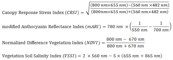
AVRIS-NG Level 2A Unrectified Reflectance (Brodrick et al. 2023) products were clipped to the study area (Figure 1) and used to derive fractional cover and vegetation and soil indices. The calculations listing the specific bands used to derive the various indices are saved within the GeoTIFF files in the ‘DESCRIPTION’ metadata field. The general formulas for deriving the indices are below. In instances where there was no band with the optimal wavelengths, the two bands on either end of this value were averaged to be used in the equation.
Fractional cover was calculated at the sub-pixel scale by using MESMA (Roberts et al., 1998). Four endmember classes were used: bare soil, green vegetation, non-photosynthetic vegetation, and water. Both 3- and 4-endmember model options were used to estimate fractional cover with at least three representative endmembers per endmember class. This calculated two or three endmember fractional covers (depending on model used) plus shade fraction for each pixel (e.g., bare soil fraction + green vegetation fraction + shade fraction).
Please see Silva et al. (2025, in press) for additional methodological details.
Data Access
These data are available through the Oak Ridge National Laboratory (ORNL) Distributed Active Archive Center (DAAC).
SHIFT: Wetland Spectra, Salinity, and Fractional Cover, Devereux Slough, CA, 2022
Contact for Data Center Access Information:
- E-mail: uso@daac.ornl.gov
- Telephone: +1 (865) 241-3952
References
Brodrick, P., R. Pavlick, M. Bernas, J.W. Chapman, R. Eckert, M. Helmlinger, M. Hess-Flores, L.M. Rios, F.D. Schneider, M.M. Smyth, M. Eastwood, R.O. Green, D.R. Thompson, K.D. Chadwick, and D.S. Schimel. 2023. SHIFT: AVIRIS-NG L2A Unrectified Reflectance. ORNL DAAC, Oak Ridge, Tennessee, USA. https://doi.org/10.3334/ORNLDAAC/2183
Gavlak, R.G., D.A. Horneck, and R.O. Miller. 2005. Soil, Plant and Water Reference Methods for the Western Region. WREP-125, 3rd edition. Western Coordinating Committee on Nutrient Management. https://www.naptprogram.org/files/napt/western-states-method-manual-2005.pdf
Rhoades, J.D. 1996. Chapter 14: Salinity: Electrical Conductivity and Total Dissolved Solids. Pp. 417-435 in D.L. Sparks, A.L. Page, P.A. Helmke, R.H. Loeppert, P.N. Soltanpour, M.A. Tabatabai, C.T. Johnston, M.E. Sumner (Eds.). Methods of Soil Analysis Part 3. Chemical Methods. SSSA Book Series. https://doi.org/10.2136/sssabookser5.3.c14
Roberts, D.A., M. Gardner, R. Church, S. Ustin, G. Scheer, and R.O. Green. 1998. Mapping chaparral in the Santa Monica Mountains using multiple endmember spectral mixture models. Remote Sensing of Environment 65:267–279. https://doi.org/10.1016/S0034-4257(98)00037-6
Roberts, D., E. Bradley, K. Roth, T. Eckmann, and C. Still. 2010. Linking physical geography education and research through the development of an environmental sensing network and project-based learning. Journal of Geoscience Education 58:262-274. https://doi.org/10.5408/1.3559887
Silva, G.D., D.A. Roberts, K.B. Byrd, K.D. Chadwick, I.J. Walker, and J.Y. King. 2025. Using imaging spectroscopy and elevation in machine learning to estimate soil salinity in intermittently tidal wetlands. Ecosphere (in press).
U.S. Geological Survey. 2020. USGS one meter x23y382 CA SoCal Wildfires B4 2018. U.S. Geological Survey. https://rockyweb.usgs.gov/vdelivery/Datasets/Staged/Elevation/1m/Projects/CA_SoCal_Wildfires_B4_2018/TIFF/