Release Date: November 4, 2011

Summary:

This data set contains forest canopy scan data from the Echidna® Validation Instrument (EVI) and field measurements data from three campaigns conducted in the United States: 2007 New England Campaign; 2008 Sierra National Forest Campaign; and 2009 New England Campaign. The New England field sites were located in Harvard Forest (Massachusetts), Howland Research Forest (Maine), and the Bartlett Experimental Forest (New Hampshire).

The objective of the research was to evaluate the ability of the EVI ground-based, scanning near-infrared lidar to retrieve stem diameter, stem count density, stand height, leaf area index, foliage profile, foliage area volume density, and other useful forest structural parameters rapidly and accurately.

The EVI scan data are Andrieu Transpose (AT) Projection images in ENVI *.img and *.hdr file pairs. There are 28 images from the 2007 New England Campaign, 40 images from the 2008 Sierra National Forest Campaign, and 54 images from the 2009 New England Campaign. There are range-weighted mean preview image files (.jpg format) for each AT Projection image.

Manual measurements of tree structural properties were made during each campaign at EVI scan locations. The field measurements are provided in one file for each campaign (.csv format). Parameters include species identification, DBH, tree height, crown base, etc. organized by field plot. 

There is also a data file (.csv format) which compares EVI derived measurements to the field measured data (DBH, stem density, basal area, biomass, and LAI) from the 2007 New England Campaign (Yao et al., 2011 and Zhao et al., 2011).

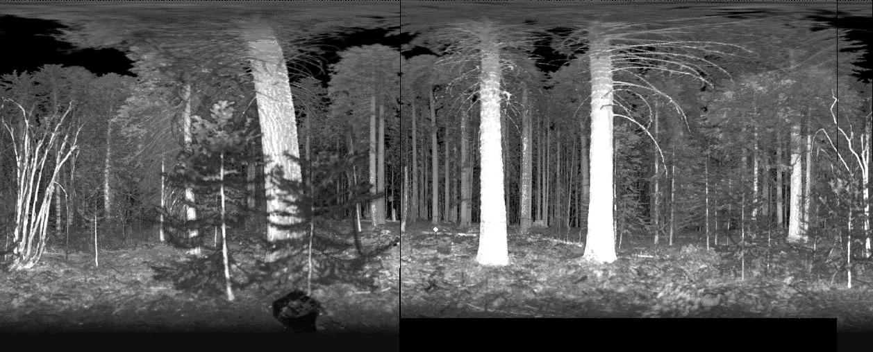
Figure 1.Example of EVI data for Bartlett Experimental Forest. Preview image of Bartlett Experimental Forest Plot 01, Center Point, 2007. The images are in a plate carrée projection that displays the data by azimuth angle (x-axis) and zenith angle (y-axis).  (2007_Bart_Plot01CP_Scan63_ND015_AT_project_Mean_range.jpg)

Data and Documentation Access:

Description and Links to Companion Files and Supplemental Information:

Get Data:  ECHIDNA Lidar Campaigns: Forest Canopy Imagery and Field Data, U.S.A., 2007-2009

Related Data Set:
Cook B., R. Dubayah, F.G. Hall, R. Nelson, J. Ranson, A.H. Strahler, P. Siqueira, M. Simard, and P. Griffith. 2011. NACP New England and Sierra National Forests Biophysical Measurements: 2008-2010. ORNL DAAC, Oak Ridge, Tennessee, USA. http:dx.doi.org/10.3334/ORNLDAAC/1046

Data Citation:

Cite this data set as follows:

Strahler, A.H., C. Schaaf, C. Woodcock, D. Jupp, D. Culvenor, G. Newnham, R. Dubayah, T. Yao, F. Zhao, and X. Yang. 2011. ECHIDNA Lidar Campaigns: Forest Canopy Imagery and Field Data, U.S.A., 2007-2009. ORNL DAAC, Oak Ridge, Tennessee, USA. http://dx.doi.org/10.3334/ORNLDAAC/1045

Table of Contents:

• 1 Data Set Overview
• 2 Data Description
• 3 Applications and Derivation
• 4 Quality Assessment
• 5 Acquisition Materials and Methods
• 6 Data Access
• 7 References

1. Data Set Overview:

Project: EOS Land Validation

The objective of this research was to prove the ability of a ground-based, scanning near-infrared lidar, the Echidna® Validation Instrument (EVI), to retrieve stem diameter, stem count density, stand height, leaf area index, foliage profile, foliage area volume density, and other useful forest structural parameters rapidly and accurately. The Echidna® instrument, built by CSIRO Australia, directs a horizontal 1,064 nm laser beam with 5 mr divergence and a pulse rate of 2 kHz to a rotating mirror at 45° incidence to scan a vertical circle, recording data from +137° to –130° zenith angles and all azimuths as the instrument revolves 180° on a tripod mount. The return signal is sampled at 2 gigasamples per second, digitizing the full scattered waveform. The shape of the return pulse distinguishes readily between hard targets (tree boles, branches) and soft targets (leaves).

To test the ability of the EVI ground-based lidar to retrieve forest structural parameters, lidar scans and manual tree measurements were acquired in 2007 and 2009 at three classic New England locations: Harvard Forest, Petersham, Massachusetts; Howland Research Forest, Howland, Maine; and Bartlett Experimental Forest, Bartlett, New Hampshire. Another field campaign was conducted in 2008 in the Sierra National Forest, California. This data set provides the results from these campaigns, both the scan imagery and the field measurements.

2. Data Description:

This data set contains forest canopy scan data from the Echidna® Validation Instrument (EVI), field measurement data from the three campaigns, and a comparison of EVI derived measurements to the field measured data from the 2007 New England Campaign.

EVI Images:

28 Andrieu Transpose (AT) Projection image files (.img) from the 2007 New England Campaign, 

40 AT Projection image files from the 2008 Sierra National Forest Campaign, and 

54 AT Projection image files from the 2009 New England Campaign. 

EVI Preview Images:

There are range-weighted mean image files (.jpg format) for each AT Projection image. See tables below of field campaign locations for preview image links.

Field Measurement Data:

• Field measurement data of tree structural properties collected during each campaign at EVI scan locations. 
• The field measurement files (.csv format) contain species identification, DBH, tree height, crown base, etc. organized by field plot and subplot.

Comparison of EVI derived measurements to the field measurements from the 2007 New England Campaign.

• Compilation of 2007 New England Campaign EVI derived plot biometric data and field measurement plot data.
• Data file (.csv format) with compiled EVI derived measurements and the field measured data (DBH, stem density,basal area, biomass, and LAI) for  the 2007 New England Campaign sites.
• Summary data tables with statistical comparisons of  EVI derived data and field measurements.

Spatial Coverage

Site: United States

Site Boundaries: (All latitude and longitude given in decimal degrees)

Site(Region)	Westernmost Longitude	Easternmost Longitude	Northernmost Latitude	Southernmost Latitude
New England, U.S.A.	-72.18222	-68.72358	45.21483	42.53097
Sierra National Forest, California, U.S.A.	-119.249	-119.0504	37.0979	36.961

The New England campaign field sites were located in Harvard Forest (Massachusetts), Howland Research Forest (Maine), and Bartlett Experimental Forest (New Hampshire). There were two field plots in each forest for a total of six plots per campaign (2007 and 2009). Two of the plots were studied in both campaign years [Harvard Forest Hemlock site (HF_HH) and Howland Forest BU Shelterwood site (HOW8)]. The New England site locations are shown in Tables 1 and 3 below. The GPS locations may not match to each other from 2007 to 2009 due to the GPS accuracy. For these sites, the 2009 GPS locations should be the most accurate. The number of subplots varied per location and campaign (See Tables 5, 8, and 10).  Table 4 is a cross reference for the various Plot IDs used for the New England sites.

The California campaign field sites were located in the Sierra National Forest. There are eight forest plots in this campaign (2008). Site locations are shown in Table 2 below.

Table 1. New England Sites, Plot Center Points, 2007

Site	Plot	Longitude***	Latitude
Harvard Forest	Plot 01	-72.18222	42.53097
Harvard Forest	Plot 02*	-72.17756	42.53828
Howland Research Forest	Plot 01**	-68.73806	45.21053
Howland Research Forest	Plot 02	-68.72358	45.20475
Bartlett Experimental Forest	Plot 01	-71.28944	44.04756
Bartlett Experimental Forest	Plot 02	-71.27	44.04756

* The Harvard Forest Plot 02 in 2007 was revisited in 2009 and designated "HF_HH".

** The Howland Research Forest Plot 01 was revisited in 2009 and designated "HOW8".

*** The GPS locations may not match to each other from 2007 to 2009 due to the GPS accuracy. For revisited sites, the 2009 GPS locations should be the most accurate.

Table 2. Sierra National Forest Site, Plot Center Points, 2008

Site	Plot	Longitude	Latitude
Sierra National Forest	Site 23	-119.249	37.0979
Sierra National Forest	Site 99	-119.1879	37.0373
Sierra National Forest	Site 168	-119.0504	36.961
Sierra National Forest	Site 301	-119.0568	36.98
Sierra National Forest	Site 305	-119.0523	36.9796
Sierra National Forest	Site 338	-119.0561	36.9703
Sierra National Forest	Site 406	-119.221	37.0959
Sierra National Forest	Site 801	-119.1085	37.0215

Table 3. New England Sites, Plot Center Points, 2009

Site	Plot	Longitude*	Latitude
Harvard Forest	HF_PH3	-72.17266	42.53665
Harvard Forest	HF_HH **	-72.17763	42.53665
Howland Research Forest	HOW7	-68.73479	45.21483
Howland Research Forest	HOW8 **	-68.73806	45.21054
Bartlett Experimental Forest	BF_38M	-71.27894	44.05432
Bartlett Experimental Forest	BF_NACP	-71.28809	44.06486

*The GPS locations may not match to each other from 2007 to 2009 due to the GPS accuracy. For revisited sites, the 2009 GPS locations should be the most accurate.

** 2009 plots samples in 2007.

Table 4.  New England Sites Plot ID cross reference table.  Note that Plot IDs changed from 2007 to 2009 and only two 2007 plots were revisited in 2009. Also note that the 2009 plots are included in the related data set, NACP New England and Sierra National Forests Biophysical Measurements: 2008-2010, and slightly different Plot IDs were used.

Site	2007 Plot ID	2007 Plot ID Description Dominant tree species or location	2009 Plot ID	2009 Plot ID Description	Biomass_ID NACP citation)
Harvard Forest	Harvard Forest Plot 01	Plot 01 Hardwood species
	Harvard Forest Plot 02	Plot 02 Hemlock trees	HF_HH	HF_HH is Hemlock plot (revisited in 2009)	Hemlock
			HF_PH3	HF_PH3 is EMS Tower plot	PH3
Howland Research Forest	Howland Research Forest Plot 01	Plot 01 Shelterwood location	HOW8	HOW8 is Boston University (BU) Shelterwood plot (revisited in 2009)	H8
	Howland Research Forest Plot 02	Plot 02 Tower location
			HOW7	HOW7 is Andrew Shelterwood plot	H7
Bartlett Experimental Forest	Bartlett Experimental Forest Plot 01	Plot 01 B2 location
	Bartlett Experimental Forest Plot 02	Plot 02 C2 location
			BF_38M	BF_38M is the site dominated by sugar maple	38M
			BF_NACP	BF_NACP is Tower site	NACP

Site Information

Harvard Forest  is an ecological research area of 1,200 ha owned and managed by Harvard University and located in Petersham, Massachusetts. The property, in operation since 1907, includes one of North America's oldest managed forests, educational, and research facilities. The forest stands are in the transition hardwoods - white pine - hemlock zone and are comprised mainly of red oak (Quercus rubra), red maple (Acer rubrum), yellow birch (Betula allleghaniensis), white birch (B. papyrifera), black birch (B. lenta), beech (Fagus grandifolia), white pine (Pinus strobus), and eastern hemlock (Tsuga canadensis). The study plots are located in the Prospect Hill tract. The soils are mainly sandy loam glacial till and are moderately to well drained. The climate is cool, moist temperate. July mean temperature is 20 C and January mean temperature -7 C. The annual mean precipitation of 1,066 mm is distributed fairly evenly throughout the year. Harvard Forest Website:  http://HarvardForest.fas.harvard.edu/.

Howland Research Forest is a 558 acre tract of mature, lowland evergreen forest located in central Maine, about 35 miles north of Bangor. The natural stands in this boreal-northern hardwood transitional forest consist of hemlock-spruce-fir, aspen-birch, and hemlock-hardwood mixtures ranging in age from 45 to 130 years. Dominant species composition includes red spruce (Picea rubens), eastern hemlock (Tsuga canadensis ), balsam fir (Abies balsamea), white pine (Pinus strobus), and northern white cedar (Thuja occidentalis). The land was designated as research forest in 1986 by the former owner, International Paper, and was purchased by Northeast Wilderness Trust in 2007, protecting the forest from any future logging activities. The terrain is flat to gently rolling with a maximum elevation of less than 68 m. Soils throughout the forest are glacial tills, acid in reaction, with low fertility and high organic composition. The climate is temperate continental. Howland Research Forest Website: http://HowlandForest.org/.

Bartlett Experimental Forest is a 1,052 ha tract within the U.S. Forest Service, White Mountain National Forest in New Hampshire. Research activities began at the Experimental Forest when it was established in 1931. Bartlett Experimental Forest extends from the village of Bartlett in the Saco River valley at 210 m to about 915 m at its upper reaches. The terrain is rolling to mountainous; aspects across the forest are primarily north and east. The primary forest cover is the sugar maple-beech-yellow birch association. The upper elevations support stands of spruce and fir. There are areas of old-growth northern hardwoods with beech (Fagus grandifolia), yellow birch (Betula allleghaniensis), sugar maple (Acer saccharum), and eastern hemlock (Tsuga canadensis) being the dominant species. Even-aged stands of red maple (Acer rubrum), paper birch (Betula papyrifera), and aspen (Populus tremuloides) occupy sites that were once cleared. Red spruce (Picea rubens) stands cover the highest slopes. Eastern white pine (Pinus strobus) is confined to the lowest elevations. The soils at the Bartlett Experimental Forest are spodosols, developed on glacial till derived from granite and gneiss. The soils are moist but, for the most part, well drained. The climate in the Bartlett area includes warm summers and cold winters with mean January temperatures of 9.8 C and mean July temperatures of 19.8 C. Mean annual precipitation is 1,300 mm, distributed throughout the year. Bartlett Experimental Forest Website: http://www.fs.fed.us/ne/durham/4155/bartlett.htm.

Sierra National Forest encompasses more than 24,000 km² between 274 m and 4,263 m in elevation on the western slope of the central Sierra Nevada in the state of California. The forest was placed under U.S. Forest Service protection and management in 1893. Distributions of species are largely governed by climate, which is strongly dependent on altitude. The biotic zones include the foothill woodland zone from 300 to 910 m (interior live oak), the lower montane zone from 910 to 2,100 m (yellow pine), the upper montane zone from 2,100 to 2,700 m (lodgepole pine/red fir), the subalpine zone from 2,700 to 2,900 m (whitebark pine), and the alpine zone from 2,900 m (above the tree line). In addition, some 1,550 km² of the forest are old growth, containing lodgepole pine (Pinus contorta) and red fir (Abies magnifica). Sierra National Forest Website:  http://fs.usda.gov/sierra.

Spatial Resolution

2007 New England Campaign Lidar scans and manual tree measurements were made at six New England forest plots, two plots at each location: Harvard Forest (Massachusetts), Howland Research Forest (Maine), and Bartlett Experimental Forest (New Hampshire) (Table 1). Each plot was 100 x 100 m square (1 ha) in size. The Echidna Validation Instrument was used to scan the center point of the square and center points of four 50 m x 50 m squares nested within the plot for a total of five scans at each site (except at Howland Research Forest Plot 2 where only three scans were made) (Table 4). Placements of the instrument were sometimes shifted by a few meters in order to avoid larger, nearby trunks or shrub crowns. Manual measurements of trees were made in circular plots around the scan point of 20 m range (or 25 m at Harv_01 site).

Figure 2. Plot layout in 2007 New England field work. At each one-hectare site, we acquired five ground-based lidar scans at the approximate locations shown.  Circles of 20-m radius show the areas around the scan points in which stems were mapped and measured as described within the text.

2008 Sierra National Forest Campaign Lidar scans and manual tree measurements were made at eight Sierra National Forest locations (Table 2). Each plot was 100 x 100 m square (1 ha) in size, with 9 subplots in each plot (Figure 3). Manual tree measurements were made in each subplot.

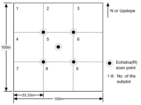
Figure 3. 2008 Sierra National Forest Campaign plot layout.

2009 New England Campaign Lidar scans and manual tree measurements were made at six New England forest plots, two plots at each location: Harvard Forest (Massachusetts), Howland Research Forest (Maine), and Bartlett Experimental Forest (New Hampshire) (Table 3). Each plot was 50 m x 50 m square, with four 25 x 25 m intensive subplots grouped together in center of the plot. Echidna® scans were made in the four corners of each plot (NW, NE, SW, and SE), in the center (C), and at N, E, S, and W locations (Figure 4A). To collect the manual tree measurements, each 50 m x 50 m plot was divided into 5 subplots (C, NW, NE, SW and SE) (Figure 4B). The central subplot was a square plot, measuring 28.53 m by 28.53 m; the other subplots were isosceles right triangle plots, with 25 m right-angle side. The numbers of stems, with DBH < 10 cm and >3 cm, were counted within a 10 m distance of the reference point in each subplot (Figure 5).

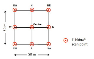
Figure: 4A

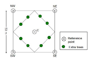
Figure: 4B

Figure 4.2009 New England Campaign (A) plot layout and Echidna® locations and (B) subplots for manual tree measurements around reference point. The "extra trees" were selected in order to register the entire stem plot map based on 13 different reference points.

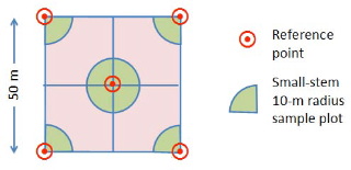
Figure 5. 2009 New England Campaign  small-stem 10-m radius sample subplots.

Temporal Coverage

2007 New England Campaign: August 1 to August 11, 2007
2008 Sierra National Forest Campaign: July 16 to July 29, 2008
2009 New England Campaign: July 23 to August 5, 2009

Temporal Resolution

Measurements were made once at the subplots listed in Tables 4-14.

Campaign Data Descriptions

2007 New England Campaign

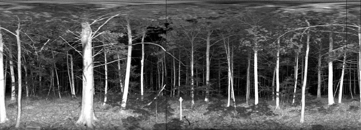
Figure 6.  Preview image of Harvard Forest Plot 02, Center Point, 2007, the images are in a plate carrée projection that displays the data by azimuth angle (x-axis) and zenith angle (y-axis). (2007_Harv_Plot02CP_Scan23_ND015_AT_project_Mean_range.jpg)

2007 New England Campaign EVI Scans

Example of Data File Structure	Image File Characteristics
EVI scan image data are distributed as *.zip files: Harv_Plot02CP_Scan23_ND015_AT_project.zip Contains: Harv_Plot02CP_ Scan23_ND015_AT_project.img Harv_Plot02CP_ Scan23_ND015_AT_project.hdr Harv_Plot02CP_ Scan23_ND015_AT_project_Mean_range.jpg Data file access: http://daac.ornl.gov/daacdata/nacp/echidna/data/	Images are ENVI .img and .hdr file pairs. Compressed files range in size from 50 - 200 MB. Image files, uncompressed, range from 1.5 - 2.5 GB. Image properties: 1257 (rows) * 454 (cols) * 1248 (bands) Andrieu Transpose (AT) Projection

Table 5.  2007 New England Campaign dates and locations of EVI scans and field measurements. Scan image file names and links to Preview images are included.

Plot_ID	Subplot	Field Measurement Date	EVI Scan Date	Longitude	Latitude	Subplot EVI Scan Image Files  (http://daac.ornl.gov/daacdata/nacp/echidna/data/)	Subplot Preview Image
Bartlett Experimental Forest Plot 01 Field Measurement Plot:  Bart_01	Center (CP)	20070809	20070809	-71.2894	44.06422	2007_Bart_Plot01CP_Scan63_ND015_AT_project.zip	2007_Bart_Plot01CP_Scan63
	Northeast (NE)	20070808	20070809	-71.2891	44.06461	2007_Bart_Plot01NE_Scan65_ND015_AT_project.zip	2007_Bart_Plot01NE_Scan65
	Northwest (NW)	20070809	20070809	-71.2897	44.0645	2007_Bart_Plot01NW_Scan61_ND015_AT_project.zip	2007_Bart_Plot01NW_Scan61
	Southeast (SE)	20070808	20070809	-71.2891	44.06386	2007_Bart_Plot01SE_Scan67_ND015_AT_project.zip	2007_Bart_Plot01SE_Scan67
	Southwest (SW)	20070809	20070809	-71.2898	44.064	2007_Bart_Plot01SW_Scan69_ND015_AT_project.zip	2007_Bart_Plot01SW_Scan69
Bartlett Experimental Forest Plot 02 Field Measurement Plot: Bart_02	Center (CP)	20070810	20070809	-71.2867	44.06422	2007_Bart_Plot02CP_Scan55_ND015_AT_project.zip	2007_Bart_Plot02CP_Scan55
	Northeast (NE)	20070810	20070809	-71.2864	44.06447	2007_Bart_Plot02NE_Scan59_ND015_AT_project.zip	2007_Bart_Plot02NE_Scan59
	Northwest (NW)	20070810	20070809	-71.2871	44.06444	2007_Bart_Plot02NW_Scan51_ND015_AT_project.zip	2007_Bart_Plot02NW_Scan51
	Southeast (SE)	20070809	20070809	-71.2864	44.06406	2007_Bart_Plot02SE_Scan57_ND015_AT_project.zip	2007_Bart_Plot02SE_Scan57
	Southwest (SW)	20070809	20070809	-71.2869	44.064	2007_Bart_Plot02SW_Scan53_ND015_AT_project.zip	2007_Bart_Plot02SW_Scan53
Harvard Forest Plot 01 Field Measurement Plot:  Harv_01	Center (CP)	20070802	20070801	-72.1821	42.53097	2007_Harv_Plot01CP_Scan21_ND015_AT_project.zip	2007_Harv_Plot01CP_Scan21
	Northeast (NE)	20070802	20070801	-72.1817	42.53119	2007_Harv_Plot01NE_Scan19_ND015_AT_project.zip	2007_Harv_Plot01NE_Scan19
	Northwest (NW)	20070801	20070801	-72.1824	42.53117	2007_Harv_Plot01NW_Scan15_ND015_AT_project.zip	2007_Harv_Plot01NW_Scan15
	Southeast (SE)	20070801	20070801	-72.1818	42.53075	2007_Harv_Plot01SE_Scan75_ND015_AT_project.zip	2007_Harv_Plot01SE_Scan75
	Southwest (SW)	20070801	20070801	-72.1823	42.53092	2007_Harv_Plot01SW_Scan17_ND015_AT_project.zip	2007_Harv_Plot01SW_Scan17
Harvard Forest Plot 02 Field Measurement Plot:  Harv_02	Center (CP)	20070803	20070802	-72.1776	42.53828	2007_Harv_Plot02CP_Scan23_ND015_AT_project.zip	2007_Harv_Plot02CP_Scan23
	Northeast (NE)	20070803	20070802	-72.1773	42.53839	2007_Harv_Plot02NE_Scan73_ND015_AT_project.zip	2007_Harv_Plot02NE_Scan73
	Northwest (NW)	20070803	20070802	-72.1779	42.53839	2007_Harv_Plot02NW_Scan25_ND015_AT_project.zip	2007_Harv_Plot02NW_Scan25
	Southeast (SE)	20070811	20070802	-72.1774	42.53789	2007_Harv_Plot02SE_Scan71_ND015_AT_project.zip	2007_Harv_Plot02SE_Scan71
	Southwest (SW)	20070803	20070802	-72.1779	42.53792	2007_Harv_Plot02SW_Scan27_ND015_AT_project.zip	2007_Harv_Plot02SW_Scan27
Howland Research Forest Plot 01 Field Measurement Plot:  How_01	Center (CP)	20070806	20070806	-68.7381	45.21053	2007_How_Plot01CP_Scan35_ND015_AT_project.zip	2007_How_Plot01CP_Scan35
	Northeast (NE)	20070806	20070806	-68.7378	45.21081	2007_How_Plot01NE_Scan33_ND015_AT_project.zip	2007_How_Plot01NE_Scan33
	Northwest (NW)	20070806	20070806	-68.7384	45.21072	2007_How_Plot01NW_Scan31_ND015_AT_project.zip	2007_How_Plot01NW_Scan31
	Southeast (SE)	20070806	20070806	-68.7378	45.21022	2007_How_Plot01SE_Scan37_ND015_AT_project.zip	2007_How_Plot01SE_Scan37
	Southwest (SW)	20070806	20070806	-68.7383	45.21036	2007_How_Plot01SW_Scan39_ND015_AT_project.zip	2007_How_Plot01SW_Scan39
Howland Research Forest Plot 02 Field Measurement Plot:  How_02	Center (CP)	20070807	20070807	-68.7403	45.20475	2007_How_Plot02CP_Scan43_ND015_AT_project.zip	2007_How_Plot02CP_Scan43
	North (NN)	20070807	20070807	-68.7403	45.20503	2007_How_Plot02NN_Scan49_ND015_AT_project.zip	2007_How_Plot02NN_Scan49
	South (SS)	20070807	20070807	-68.7403	45.20436	2007_How_Plot02SS_Scan41_ND015_AT_project.zip	2007_How_Plot02SS_Scan41

2007 New England Campaign Field Measurement Data

Plot level field measurements data are provided in a single ASCII file in comma-separated-value (.csv) format:  ne_2007_forest_field_data.csv.

Table 6. Column headings in the field measurement file for the 2007 New England Campaign.

COLUMN HEADINGS	FORMAT TYPE	UNITS	SIGNIFICANT DIGITS	MISSING CODE	DESCRIPTION
Date	Char	none	none	none	YYYYMMDD (YearMonthDay)
Site	Char	none	none	none	Name of site
Plot_ID	Char	none	none	none	Harv_01/02 are the plots in Harvard Forest Bart_01/02 are the plots in Bartlett Experimental Forest How_01/02 are the plots in Howland Research Forest
Subplot_ID	Char	none	none	none	NW, NE, CP, SW, SE, NN and SS are abbreviation for northwest, northeast, central, southwest, southeast, north and south subplot in each plot.
Tree_no	Integer	none	none	none	The ID number of the tree in each subplot.
Species	Char	none	none	none	Common name of living tree species.
DBH	Float	cm	1	-9999	Diameter Breast Height.
Distance	Float	meter	1	-9999	The distance of the tree from the reference point of the subplot. In this data set, the reference point is the center of the subplot.
Bearing1	Float	decimal degrees	1	-9999	The bearing of the tree from the reference point of the subplot. In this data set, the reference point is the center of the subplot.
Tree_height	Float	meter	1	-9999	The height from ground to the top of the tree.
Crown_base	Float	meter	1	-9999	The height from ground to the bottom of the tree crown.
OCCL	Char	none	none	none	The tree is tallied as visible (V), partly occluded (P) or fully occluded(O) from the plot center.
CR_P	Char	none	none	none	Crown position of the tree, such as dominant (D), co-dominant (C),intermediate (I), suppressed (S), or dead (Dead).
Radius1	Float	meter	3	-9999	The crown radius in one direction.
Radius2	Float	meter	3	-9999	The crown radius in the direction perpendicular to previous one (Radius1).
Notes	Char	none	none	none	The notes were made if the tallied tree is also in other plots, or if the tree has some special properties. For example, the note “Bart_01_NE-30” associated with data for Bart_01 CP tree number 19 means that Bart_01 NE tree number 30 and Bart_01 CP tree number 19 are the same tree.

Note: ¹Bearing is relative to magnetic north. It is the bearing of the tree from the reference point in the plot.

Sample of field measurement file for 2007 New England Campaign

Date,Site,Plot_ID,Subplot_ID,Tree_no,Species,DBH,Distance,Bearing,Tree_height,Crown_base,OCCL,CR_P,Radius1,Radius2,Notes 20070809,Bartlett_Forest,Bart_01,CP,19,Beech,11,18,38,-9999,-9999,O,I,-9999,-9999,Bart_01_NE-30 20070809,Bartlett_Forest,Bart_01,CP,18,Hemlock,11.7,18.8,42,-9999,-9999,O,S,-9999,-9999,Bart_01_NE-31 20070809,Bartlett_Forest,Bart_01,CP,17,YellowBirch,21.8,18.5,46,-9999,-9999,O,C,-9999,-9999,Bart_01_NE-32  ...

2008 Sierra National Forest Campaign

Figure 7. Preview image of Sierra National Forest Plot 406,Center Point, 2008. The images are in a plate carrée projection that displays the data by azimuth angle (x-axis) and zenith angle (y-axis). (2008_Site406_Centre_Scan49_ND015_AT_project_Mean_range2.jpg)

2008 Sierra National Forest Campaign EVI Scans

Table 7. Dates and locations of field measurements and EVI scans during the 2008 Sierra National Forest Campaign

Plot_ID	Field Measurement Date	EVI Scan Date	Longitude	Latitude
23	20080729	20080726	-119.249	37.0979
99	20080716	20080717	-119.1879	37.0373
168	20080721	20080722	-119.0504	36.961
301	20080719	20080721	-119.0568	36.98
305	20080718	20080717	-119.0523	36.9796
338	20080719	20080723	-119.0561	36.9703
406	20080726	20080725	-119.221	37.0959
801	20080723	20080724	-119.1085	37.0215

Example of Data File Structure	Image File Characteristics
EVI scan image data are distributed as *.zip files: 2008_Site023_Centre_Scan57_ND015_AT_project.zip Contains: Site023_Centre_Scan57_ND015_AT_project.img Site023_Centre_Scan57_ND015_AT_project.hdr Site023_Centre_Scan57_ND015_AT_project_Mean_range2.jpg Data file access:  http://daac.ornl.gov/daacdata/nacp/echidna/data/	Images are ENVI .img and .hdr file pairs. Compressed files range in size from 50 - 200 MB. Image files, uncompressed, range from 1.5 - 2.5 GB. Image properties: 1257 (rows) * 508 (cols) * 1915 (bands) Andrieu Transpose (AT) Projection

Table 8.  2008 Sierra National Forest Campaign locations of EVI scans. Scan image file names and links to Preview images are included.

Plot_ID	Subplot	Subplot EVI Scan Image Files  (http://daac.ornl.gov/daacdata/nacp/echidna/data/)	Subplot Preview Image
23	Centre	2008_Site023_Centre_Scan57_ND015_AT_project.zip	2008_Site023_Centre_Scan57
	LLcorner	2008_Site023_LLcorner_Scan62_ND015_AT_project.zip	2008_Site023_LLcorner_Scan62
	LRcorner	2008_Site023_LRcorner_Scan61_ND015_AT_project.zip	2008_Site023_LRcorner_Scan61
	ULcorner	2008_Site023_ULcorner_Scan59_ND015_AT_project.zip	2008_Site023_ULcorner_Scan59
	URcorner	2008_Site023_URcorner_Scan60_ND015_AT_project.zip	2008_Site023_URcorner_Scan60
99	Centre	2008_Site99_Centre_Scan11_ND015_AT_project.zip	2008_Site99_Centre_Scan11
	LLcorner	2008_Site99_LLcorner_Scan09_ND015_AT_project.zip	2008_Site99_LLcorner_Scan09
	LRcorner	2008_Site99_LRcorner_Scan05_ND015_AT_project.zip	2008_Site99_LRcorner_Scan05
	ULcorner	2008_Site99_ULcorner_Scan13_ND015_AT_project.zip	2008_Site99_ULcorner_Scan13
	URcorner	2008_Site99_URcorner_Scan02_ND015_AT_project.zip	2008_Site99_URcorner_Scan02
168	Centre	2008_Site168_Centre_Scan31_ND015_AT_project.zip	2008_Site168_Centre_Scan31
	LLcorner	2008_Site168_LLcorner_Scan34_ND015_AT_project.zip	2008_Site168_LLcorner_Scan34
	LRcorner	2008_Site168_LRcorner_Scan35_ND015_AT_project.zip	2008_Site168_LRcorner_Scan35
	ULcorner	2008_Site168_ULcorner_Scan33_ND015_AT_project.zip	2008_Site168_ULcorner_Scan33
	URcorner	2008_Site168_URcorner_Scan36_ND015_AT_project.zip	2008_Site168_URcorner_Scan36
301	Centre	2008_Site301_Centre_Scan24_ND015_AT_project.zip	2008_Site301_Centre_Scan24
	LLcorner	2008_Site301_LLcorner_Scan27_ND015_AT_project.zip	2008_Site301_LLcorner_Scan27
	LRcorner	2008_Site301_LRcorner_Scan30_ND015_AT_project.zip	2008_Site301_LRcorner_Scan30
	ULcorner	2008_Site301_ULcorner_Scan26_ND015_AT_project.zip	2008_Site301_ULcorner_Scan26
	URcorner	2008_Site301_URcorner_Scan23_ND015_AT_project.zip	2008_Site301_URcorner_Scan23
305	Centre	2008_Site305_Centre_Scan17_ND015_AT_project.zip	2008_Site305_Centre_Scan17
	LLcorner	2008_Site305_LLcorner_Scan21_ND015_AT_project.zip	2008_Site305_LLcorner_Scan21
	LRcorner	2008_Site305_LRcorner_Scan22_ND015_AT_project.zip	2008_Site305_LRcorner_Scan22
	ULcorner	2008_Site305_ULcorner_Scan18_ND015_AT_project.zip	2008_Site305_ULcorner_Scan18
	URcorner	2008_Site305_URcorner_Scan20_ND015_AT_project.zip	2008_Site305_URcorner_Scan20
338	Centre	2008_Site338_Centre_Scan37_ND015_AT_project.zip	2008_Site338_Centre_Scan37
	LLcorner	2008_Site338_LLcorner_Scan42_ND015_AT_project.zip	2008_Site338_LLcorner_Scan42
	LRcorner	2008_Site338_LRcorner_Scan41_ND015_AT_project.zip	2008_Site338_LRcorner_Scan41
	ULcorner	2008_Site338_Scan40_URcorner_ND015_AT_project.zip	2008_Site338_ULcorner_Scan39
	URcorner	2008_Site338_ULcorner_Scan39_ND015_AT_project.zip	2008_Site338_URcorner_Scan40
406	Centre	2008_Site406_Centre_Scan49_ND015_AT_project.zip	2008_Site406_Centre_Scan49
	LLcorner	2008_Site406_LLcorner_Scan56_ND015_AT_project.zip	2008_Site406_LLcorner_Scan56
	LRcorner	2008_Site406_LRcorner_Scan55_ND015_AT_project.zip	2008_Site406_LRcorner_Scan55
	ULcorner	2008_Site406_ULcorner_Scan53_ND015_AT_project.zip	2008_Site406_ULcorner_Scan53
	URcorner	2008_Site406_URcorner_Scan54_ND015_AT_project.zip	2008_Site406_URcorner_Scan54
801	Centre	2008_Site801_Centre_Scan45_ND015_AT_project.zip	2008_Site801_Centre_Scan45
	LLcorner	2008_Site801_LLcorner_Scan47_ND015_AT_project.zip	2008_Site801_LLcorner_Scan47
	LRcorner	2008_Site801_LRcorner_Scan48_ND015_AT_project.zip	2008_Site801_LRcorner_Scan48
	ULcorner	2008_Site801_ULcorner_Scan44_ND015_AT_project.zip	2008_Site801_ULcorner_Scan44
	URcorner	2008_Site801_URcorner_Scan43_ND015_AT_project.zip	2008_Site801_URcorner_Scan43

Plot level field measurements data are provided in a single ASCII file in comma-separated-value (.csv) format:  sierra_2008_forest_field_data.csv.

Table 9. Column headings in field measurements file for 2008 Sierra National Forest Campaign.

COLUMN HEADINGS	FORMAT TYPE	UNITS	SIGNIFICANT DIGITS	MISSING CODE	DESCRIPTION
Date	Char	none	none	none	YYYYMMDD (YearMonthDay)
Site	Char	none	none	none	Name of site.
Plot_ID	Char	none	none	none	There are eight plots totally with the name of number: 23, 99, 168, 301, 305, 338, 406, 801.
Subplot_ID	Char	none	none	none	There are 9 subplots within each plot identified with numbers from 1 to 9. Figure 1 shows the locations of the subplots.
Tree_no	Integer	none	none	none	The ID number of the tree in each subplot
Species1	Char	none	none	none	Tree species code. The code “none” indicates that the tree was not identified to species. See Table 18.
Status	Char	none	none	none	L means the tree is live, and D means the tree is dead.
DBH	Float	cm	1	-9999	Diameter Breast Height
Biomass_Jenkins	Float	megagrams (Mg)	???	-9999	Biomass was calculated using the equations from Jenkins et al. 2004.(NACP citation)
Distance	Float	meter	1	-9999	The distance from the front of the tree to the reference point in the plot.
Bearing2	Float	degrees	1	-9999	The bearing of the tree from the reference point in the plot.
Tree_height	Float	meter	1	-9999	The height from ground to the top of the tree.
Crown_base	Float	meter	1	-9999	The height from ground to the bottom of the tree crown.
Crown_along_slope	Float	meter	1	-9999	The crown diameter along the slope direction.
Crown_across_slope	Float	meter	1	-9999	The crown diameter across the slope direction.
Crown_form	Char	none	none	none	The shape of the crown.
Notes	Char	none	none	none	Thenotes were made if the tree has some special properties.

Notes: ¹The code list for the parameter species. The species codes are derived from the USDA NRCS PLANTS Database at http://plants.usda.gov/. The complete list is available for download at http://plants.usda.gov/dl_all.html.

²Bearing is relative to magnetic north. It is the bearing of the tree from the reference point in the plot.

Tree species code list for 2008 Sierra National Forest Campaign

Species_code	Species Name	Common Name
ABCO	Abies concolor	White Fir
ABMA	Abies magnifica	Red Fir
FRLA	Fraxinuslatifolia	Oregon ash
SEGI	Sequoiadendron giganteum	Giant Sequoia
LIDE	Libocedrus decurrens	Incense cedar
PICO	Pinus contorta	Lodgepole pine
PIJE	Pinus jeffreyi	Jeffrey pine
PILA	Pinus lambertiana	Sugar pine
PIMO	Pinus monticola	Western white pine
PIPO	Pinus ponderosa	Ponderosa pine
PISA	Pinus sabiniana	Gray pine
POTR	Populus tremuloides	Trembling aspen
PREM	Prunus emarginate	Bitter cherry
PRSU	Prunus subcordata	Sierra plum
PRVI	Prunus virginiana	Western chokecherry
QUCH	Quercus chrysolepis	Canyon live oak
QUKE	Quercus kellogii	Black oak
UNK	unknown species

Sample of field measurement file for 2008 Sierra National Forest Campaign

Date,Site,Plot_ID,Subplot_ID,Tree_no,Species,Status,DBH,Distance,Bearing,Tree_height,Crown_base, Crown_along_slope,Crown_cross_slope,Crown_form,Notes none,none,none,none,none,none,none,cm,meter,decimal_degrees,meter,meter,meter,meter,none,none 20080729,Sierra_National_Forest,23,1,1,PIJE,L,70.1,-9999,-9999,26.39,-9999,-9999,-9999,none,none 20080729,Sierra_National_Forest,23,1,2,PIJE,L,28,-9999,-9999,-9999,-9999,-9999,-9999,none,none 20080729,Sierra_National_Forest,23,1,4,PIJE,L,69.8,-9999,-9999,-9999,-9999,-9999,-9999,none,none ...

2009 New England Campaign

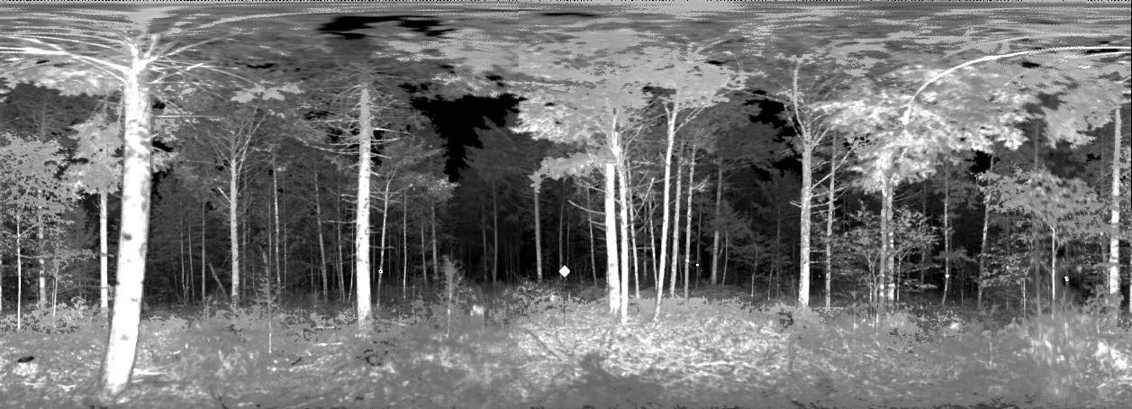
Figure 8. Preview image of Howland Forest Plot, HOW8, Center Point, 2009. The images are in a plate carréeprojection that displays the data by azimuth angle (x-axis) and zenith angle (y-axis). (2009_HOW8_Scan_04_Centre_AT_project_Mean_range.jpg)

2009 New England Campaign EVI Scans

Example of Data File Structure	Image File Characteristics
EVI scan image data are distributed as *.zip files: 2009_HF_PH3_Scan_09_NW_AT_project.zip Contains: HF_PH3_Scan_09_NW_AT_project.img HF_PH3_Scan_09_NW_AT_project.img.hdr HF_PH3_Scan_09_NW_AT_project_Mean_range.jpg Data file access:  http://daac.ornl.gov/daacdata/nacp/echidna/data/	Images are ENVI .img and .hdr file pairs. Compressed files range in size from 50 - 200 MB. Image files, uncompressed, range from 1.5 - 2.5 GB. Image properties: 1257 (rows) * 454 (cols) * 1515 (bands) Andrieu Transpose (AT) Projection

Table 10.  2009 New England Campaign dates and locations of EVI scans and field measurements. Scan image file names and links to Preview images are included.

Location	Plot_ID	Subplot_ID	Field Measurement Date	Scan_ID	EVI Scan Date	Longitude	Latitude	Subplot EVI Scan Image Files  (http://daac.ornl.gov/daacdata/nacp/echidna/data/)	Subplot Preview Image
Harvard Forest	HF_PH3	N		Scan_01_N	20090726	-72.17276	42.53675	2009_HF_PH3_Scan_01_N_AT_project.zip	2009_HF_PH3_Scan_01_N
Harvard Forest	HF_PH3	NE	20090723	Scan_02_NE	20090726	-72.17238	42.53669	2009_HF_PH3_Scan_02_NE_AT_project.zip	2009_HF_PH3_Scan_02_NE
Harvard Forest	HF_PH3	E		Scan_03_E	20090726	-72.17246	42.53658	2009_HF_PH3_Scan_03_E_AT_project.zip	2009_HF_PH3_Scan_03_E
Harvard Forest	HF_PH3	SE	20090723	Scan_04_SE	20090726	-72.17244	42.53639	2009_HF_PH3_Scan_04_SE_AT_project.zip	2009_HF_PH3_Scan_04_SE
Harvard Forest	HF_PH3	S		Scan_05_S	20090726	-72.17274	42.53629	2009_HF_PH3_Scan_05_S_AT_project.zip	2009_HF_PH3_Scan_05_S
Harvard Forest	HF_PH3	SW	20090723	Scan_06_SW	20090726	-72.17304	42.536	2009_HF_PH3_Scan_06_SW_AT_project.zip	2009_HF_PH3_Scan_06_SW
Harvard Forest	HF_PH3	C	20090723	Scan_07_Centre	20090726	-72.17266	42.53665	2009_HF_PH3_Scan_07_Centre_AT_project.zip	2009_HF_PH3_Scan_07_Centre
Harvard Forest	HF_PH3	W		Scan_08_W	20090726	-72.17306	42.53666	2009_HF_PH3_Scan_08_W_AT_project.zip	2009_HF_PH3_Scan_08_W
Harvard Forest	HF_PH3	NW	20090723	Scan_09_NW	20090726	-72.17297	42.53688	2009_HF_PH3_Scan_09_NW_AT_project.zip	2009_HF_PH3_Scan_09_NW
Harvard Forest	HF_HH	C	20090726	Scan_01_Centre	20090725	-72.17763	42.53819	2009_HF_HH_Scan_01_Centre_AT_project.zip	2009_HF_HH_Scan_01_Centre
Harvard Forest	HF_HH	NE	20090726	Scan_02_NE	20090725	-72.17717	42.53833	2009_HF_HH_Scan_02_NE_AT_project.zip	2009_HF_HH_Scan_02_NE
Harvard Forest	HF_HH	SE	20090726	Scan_03_SE	20090725	-72.17736	42.53781	2009_HF_HH_Scan_03_SE_AT_project.zip	2009_HF_HH_Scan_03_SE
Harvard Forest	HF_HH	S		Scan_04_S	20090725	-72.17773	42.53786	2009_HF_HH_Scan_04_S_AT_project.zip	2009_HF_HH_Scan_04_S
Harvard Forest	HF_HH	SW	20090726	Scan_05_SW	20090725	-72.17793	42.53788	2009_HF_HH_Scan_05_SW_AT_project.zip	2009_HF_HH_Scan_05_SW
Harvard Forest	HF_HH	W		Scan_06_W	20090725	-72.17784	42.53817	2009_HF_HH_Scan_06_W_AT_project.zip	2009_HF_HH_Scan_06_W
Harvard Forest	HF_HH	NW	20090726	Scan_07_NW	20090725	-72.17779	42.53839	2009_HF_HH_Scan_07_NW_AT_project.zip	2009_HF_HH_Scan_07_NW
Harvard Forest	HF_HH	N		Scan_08_N	20090725	-72.17749	42.53833	2009_HF_HH_Scan_08_N_AT_project.zip	2009_HF_HH_Scan_08_N
Harvard Forest	HF_HH	E		Scan_09_E	20090725	-72.17731	42.53798	2009_HF_HH_Scan_09_E_AT_project.zip	2009_HF_HH_Scan_09_E
Howland Forest	HOW7	S		Scan_01_S	20090801	N/A	N/A	2009_HOW7_Scan_01_S_AT_project.zip	2009_HOW7_Scan_01_S
Howland Forest	HOW7	SW	20090801	Scan_02_SW	20090801	-68.73504	45.21456	2009_HOW7_Scan_02_SW_AT_project.zip	2009_HOW7_Scan_02_SW
Howland Forest	HOW7	W		Scan_03_W	20090801	N/A	N/A	2009_HOW7_Scan_03_W_AT_project.zip	2009_HOW7_Scan_03_W
Howland Forest	HOW7	NW	20090801	Scan_04_NW	20090801	-68.7351	45.215	2009_HOW7_Scan_04_NW_AT_project.zip	2009_HOW7_Scan_04_NW
Howland Forest	HOW7	N		Scan_05_N	20090801	N/A	N/A	2009_HOW7_Scan_05_N_AT_project.zip	2009_HOW7_Scan_05_N
Howland Forest	HOW7	NE	20090801	Scan_06_NE	20090801	-68.73458	45.2151	2009_HOW7_Scan_06_NE_AT_project.zip	2009_HOW7_Scan_06_NE
Howland Forest	HOW7	E		Scan_07_E	20090801	-68.73414	45.2149	2009_HOW7_Scan_07_E_AT_project.zip	2009_HOW7_Scan_07_E
Howland Forest	HOW7	C	20090801	Scan_08_Centre	20090801	-68.73479	45.21483	2009_HOW7_Scan_08_Centre_AT_project.zip	2009_HOW7_Scan_08_Centre
Howland Forest	HOW7	SE	20090801	Scan_09_SE	20090801	-68.73446	45.21468	2009_HOW7_Scan_09_SE_AT_project.zip	2009_HOW7_Scan_09_SE
Howland Forest	HOW8	NW	20090801	Scan_01_NW	20090731	N/A	N/A	2009_HOW8_Scan_01a_NW_AT_project.zip	2009_HOW8_Scan_01a_NW
Howland Forest	HOW8	N		Scan_02_N	20090731	N/A	N/A	2009_HOW8_Scan_02_N_AT_project.zip	2009_HOW8_Scan_02_N
Howland Forest	HOW8	NE	20090801	Scan_03_NE	20090731	N/A	N/A	2009_HOW8_Scan_03_NE_AT_project.zip	2009_HOW8_Scan_03_NE
Howland Forest	HOW8	C	20090801	Scan_04_Centre	20090731	-68.73806	45.21054	2009_HOW8_Scan_04_Centre_AT_project.zip	2009_HOW8_Scan_04_Centre
Howland Forest	HOW8	E		Scan_05_E	20090731	N/A	N/A	2009_HOW8_Scan_05_E_AT_project.zip	2009_HOW8_Scan_05_E
Howland Forest	HOW8	W		Scan_06_W	20090731	N/A	N/A	2009_HOW8_Scan_06_W_AT_project.zip	2009_HOW8_Scan_06_W
Howland Forest	HOW8	SW	20090801	Scan_07_SW	20090731	N/A	N/A	2009_HOW8_Scan_07_SW_AT_project.zip	2009_HOW8_Scan_07_SW
Howland Forest	HOW8	S		Scan_08_S	20090731	N/A	N/A	2009_HOW8_Scan_08_S_AT_project.zip	2009_HOW8_Scan_08_S
Howland Forest	HOW8	SE	20090801	Scan_09_SE	20090731	N/A	N/A	2009_HOW8_Scan_09_SE_AT_project.zip	2009_HOW8_Scan_09_SE
Bartlett Forest	BF_38M	C	20090803	Scan_01_Centre	20090805	-71.27894	44.05432	2009_BF_38M_Scan_01_Centre_AT_project.zip	2009_BF_38M_Scan_01_Centre
Bartlett Forest	BF_38M	NW	20090803	Scan_02_NW	20090805	-71.2792	44.05455	2009_BF_38M_Scan_02_NW_AT_project.zip	2009_BF_38M_Scan_02_NW
Bartlett Forest	BF_38M	NE	20090803	Scan_03_NE	20090805	-71.27875	44.05454	2009_BF_38M_Scan_03_NE_AT_project.zip	2009_BF_38M_Scan_03_NE
Bartlett Forest	BF_38M	SE	20090803	Scan_04_SE	20090805	-71.27872	44.05405	2009_BF_38M_Scan_04_SE_AT_project.zip	2009_BF_38M_Scan_04_SE
Bartlett Forest	BF_38M	S		Scan_05_S	20090805	-71.2791	44.05406	2009_BF_38M_Scan_05_S_AT_project.zip	2009_BF_38M_Scan_05_S
Bartlett Forest	BF_38M	W		Scan_06_W	20090805	-71.27929	44.05433	2009_BF_38M_Scan_06_W_AT_project.zip	2009_BF_38M_Scan_06_W
Bartlett Forest	BF_38M	N		Scan_07_N	20090805	-71.27898	44.05455	2009_BF_38M_Scan_07_N_AT_project.zip	2009_BF_38M_Scan_07_N
Bartlett Forest	BF_38M	E		Scan_08_E	20090805	-71.27869	44.05432	2009_BF_38M_Scan_08_E_AT_project.zip	2009_BF_38M_Scan_08_E
Bartlett Forest	BF_38M	SW	20090803	Scan_09_SW	20090805	-71.27924	44.05408	2009_BF_38M_Scan_09_SW_AT_project.zip	2009_BF_38M_Scan_09_SW
Bartlett Forest	BF_NACP	E		Scan_01_E	20090804	-71.2878	44.06499	2009_BF_NACP_Scan_01_E_AT_project.zip	2009_BF_NACP_Scan_01_E
Bartlett Forest	BF_NACP	SE	20090805	Scan_02_SE	20090804	-71.28771	44.06474	2009_BF_NACP_Scan_02_SE_AT_project.zip	2009_BF_NACP_Scan_02_SE
Bartlett Forest	BF_NACP	NE	20090805	Scan_03_NE	20090804	-71.28796	44.06513	2009_BF_NACP_Scan_03_NE_AT_project.zip	2009_BF_NACP_Scan_03_NE
Bartlett Forest	BF_NACP	N		Scan_04_N	20090804	-71.28828	44.06512	2009_BF_NACP_Scan_04_N_AT_project.zip	2009_BF_NACP_Scan_04_N
Bartlett Forest	BF_NACP	C	20090805	Scan_05_Centre	20090804	-71.28809	44.06486	2009_BF_NACP_Scan_05_Centre_AT_project.zip	2009_BF_NACP_Scan_05_Centre
Bartlett Forest	BF_NACP	S		Scan_06_S	20090804	-71.28798	44.06469	2009_BF_NACP_Scan_06_S_AT_project.zip	2009_BF_NACP_Scan_06_S
Bartlett Forest	BF_NACP	SW	20090805	Scan_07_SW	20090804	-71.28831	44.06458	2009_BF_NACP_Scan_07_SW_AT_project.zip	2009_BF_NACP_Scan_07_SW
Bartlett Forest	BF_NACP	W		Scan_08_W	20090804	-71.28839	44.06478	2009_BF_NACP_Scan_08_W_AT_project.zip	2009_BF_NACP_Scan_08_W
Bartlett Forest	BF_NACP	NW	20090805	Scan_09_NW	20090804	-71.2885	44.06503	2009_BF_NACP_Scan_09_NW_AT_project.zip	2009_BF_NACP_Scan_09_NW

Plot level field measurement data are provided in a single ASCII file in comma-separated-value (.csv) format: ne_2009_forest_field_data.csv.

Table 11. Column headings in field measurements file for 2009 New England Campaign

COLUMN HEADINGS	FORMAT TYPE	UNITS	SIGNIFICANT DIGITS	MISSING CODE	DESCRIPTION
Date	Char	None	None	NA	YYYYMMDD(YearMonthDay)
Site	Char	None	None	NA	Harvard Forest site is in MA; Howland Forest site is in ME; Bartlett Forest site is in NH.
Plot_ID	Char	None	None	NA	HF_PH3 is Harvard Forest EMS Tower plot; HF_HH is Harvard Forest Hemlock plot (revisited); HOW7 is Howland Forest Andrew Shelterwood plot; HOW8 is Howland Forest BU Shelterwood plot (revisited); BF_38M is plot in Bartlett Forest dominated by sugar maple; BF_NACP is Bartlett Forest Tower site.
Subplot_ID	Char	None	None	NA	Each plot is divided into 5 subplots based on different reference point: C, NW, NE, SW and SE (Figure 2).
Tree_no	Integer	None	1	-9999	The number of the tree in each subplot.
Species1	Char	None	None	NA	Tree species for each tree.
Status	Char	None	None	NA	The tree is live (L) or dead (D).
DBH	Float	centimeter	1	-9999	Diameter at Breast Height (about 1.3 m)
Distance	Float	meter	1	-9999	The distance of the tree from the reference point of the subplot.
Bearing2	Float	decimal degree	1	-9999	The bearing of the tree from the reference point of the subplot.
Tree_height	Float	meter	1	-9999	Tree height, height to crown base and crown dimensions (the longest axis and the perpendicular one), were measured on every tenth tree.
Crown_base	Float	meter	1	-9999	The height from the ground to the base of live tree crown.
Crown_diameter_max	Float	meter	2	-9999	The max crown diameter.
Crown_diameter_cross	Float	meter	2	-9999	The crown diameter in the cross direction.
Notes	Char	None	None	NA	Field observations
Cross-ref_distance3	Float	meter	1	-9999	The distance from the central reference point to “extra” trees in the subplot NW/NE/SW/SE (Figure 2).See Methods Section for explanation.
Cross-ref_bearing3	Float	decimal degree	1	-9999	The bearing from the central reference point to “extra” trees in the subplot NW/NE/SW/SE (Figure 2). See Methods Section for explanation.

Sample of field measurements file for 2009 New England Campaign

Date,Site,Plot_ID,Subplot_ID,Tree_no,Species,Status,DBH,Distance,Bearing,Tree_height,Crown_base, Crown_diameter_max,Crown_diameter_cross,Notes,Cross-ref_distance,Cross-ref_bearing none,none,none none none none none cm m degrees meter meter meter meter none degrees degrees 20090723,Harvard_Forest,HF_PH3,C,1,ACRU,L,29,9.5,89,15.2,11,8.4,7.9,none,-9999,-9999 20090723,Harvard_Forest,HF_PH3,C,2,ACRU,L,27,11.7,103,-9999,-9999,-9999,-9999,none,-9999,-9999 20090723,Harvard_Forest,HF_PH3,C,3,ACRU,L,64,13.5,103.5,-9999,-9999,-9999,-9999,none,-9999,-9999 ...

Field Measurements Results and EVI Derived Data Comparison, New England 2007

This data file contains results of field measurements (DBH, stand density, basal area, biomass, and LAI) and comprable EVI scan derived values (EVI_*)  from the 2007 New England Campaign.  Data are provided in one ASCII file in comma-separated-value (.csv) format:   ne_2007_echidna_field_comparisons.csv

Tables 13, 14, and 15 contain various summary statistics of comparitive analyses of manual field measurements of forest canopy parameters to those derived from the Echidna scan data.  Source: Yao et al., 2011.

Table 12. Column headings in comparative analyses data file for 2007 New England Campaign.

COLUM NNAME	FORMAT TYPE	UNITS	SIGNIFICANT DIGITS	DESCRIPTION
DATE	Char	None	None	YYYYMMDD (YearMonthDay)
PLOT_ID	Char	none	none	Harv_01/02 are the plots in Harvard Forest Bart_01/02 are the plots in Bartlett Experimental Forest How_01/02 are the plots in Howland Research Forest
SUBPLOT_ID	Char	none	none	NW, NE, CP, SW, SE, NN and SS are abbreviation for northwest, northeast,central, southwest, southeast, north and south subplot in each plot. ALL means the entire plot.
FIELD_DBH	Float	meter	3	Mean Diameter Breast Height
EVI_DBH	Float	meter	3	Diameter Breast Height
FIELD_STEMDEN	Integer	stems per hectare (stem/ha)	0	Total stem count density
EVI_STEMDEN	Integer	stems per hectare(stem/ha)	0	Total stem count density
FIELD_BA	Float	m2per hectare	2	Mean basal area of plot or subplot
EVI_BA	Float	m2 per hectare	2	Mean basal area of plot or subplot
FIELD_BIOMASS	Float	ton per hectare	2	Mean above ground woody biomass
EVI_BIOMASS	Float	ton per hectare	2	Mean above ground woody biomass
LAI_2000	Float	m2/m2	2	One sided green leaf area per unit ground area in broadleaf canopies, or as the projected needle leaf area per unit ground area in needle canopies from LAI_2000 data
HEMI_LAI	Float	m2/m2	2	One sided green leaf area per unit ground area in broadleaf canopies, or as the projected needle leaf area per unit ground area in needle canopies from Hemispherical photographs data
EVI_LAI_REGRE	Float	m2/m2	2	One sided green leaf area per unit ground area in broadleaf canopies, or as the projected needle leaf area per unit ground area in needle canopies from EVI data. It's calculated by a simple regression method.
EVI_LAI_HINGE	Float	m2/m2	2	One sided green leaf area per unit ground area in broadleaf canopies, or as the projected needle leaf area per unit ground area in needle canopies from EVI data. It's calculated by "hinge angle" method.
DOMI_SPECIES	Char	none	none	Common name of dominant tree species

Sample of results file for comparative analyses file for 2007 New England Campaign.

DATE,PLOT_ID,SUBPLOT_ID,FIELD_DBH,EVI_DBH,FIELD_STEMDEN,EVI_STEMDEN,FIELD_BA, EVI_BA,Field_BIOMASS,EVI_BIOMASS,LAI_2000,HEMI_LAI,EVI_LAI_REGRE,EVI_LAI_HINGE, DOMI_SPECIES none,none,none,meter,meter,stem/ha,stem/ha,m2/ha,m2/ha,ton/ha,ton/ha,m2/m2,m2/m2,m2/m2,m2/m2,none 20070808-20070809,Bart_01,ALL,0.166,0.161,1432,1467,44.96,45.49,254.06,240.02,4.76, 3.92,4.6,4.95,RedMaple YellowBirch 20070809,Bart_01,CP,0.173,0.152,1472,1400,47.7,42.24,284.73,232,4.89,4.16,4.3,4.55,RedMaple WhiteAsh 20070808,Bart_01,NE,0.176,0.2,1289,1265,44,48.09,249.2,251.4,4.52,3.7,4.56,4.95,RedMaple YellowBirch ...

Table 13. Summary of stand attributes, New England forest sites, 2007¹

		Harvard		Howland		Bartlett		Site R2	Plot R2	95% Confidence Interval of Intercept (Plot level)	95% Confidence Interval of Slope (Plot level)
		Plot 01	Plot 02	Plot 01	Plot 02	Plot 01	Plot 02
Arithmetic mean of DBH (m)	Field	0.168 ± 0.008	0.198 ± 0.006	0.156 ± 0.015	0.127 ± 0.009	0.166 ± 0.007	0.148 ± 0.007	0.936	0.479	(-0.107,0.015)	(0.902,1.642)
	EVI	0.170 ± 0.016	0.200 ± 0.002	0.165 ± 0.011	0.118 ± 0.009	0.161 ± 0.014	0.134 ± 0.011
Stem count Density (trees/ha)	Field	1020 ± 72	1284 ± 98	1017 ± 179	3281 ± 353	1432 ± 67	1485 ± 27	0.999	0.902	(-211.1, 211.1)	(0.901,1.162)
	EVI	1105 ± 71	1331 ± 130	1042 ± 179	3341 ± 494	1467 ± 73	1549 ± 84
Basal area (m2/ha)	Field	37.46 ± 1.65	55.48 ± 1.96	26.50 ± 0.86	55.36 ± 3.08	44.96 ± 1.55	40.66 ± 3.21	0.938	0.656	(-11.807,9.386)	(0.780,1.263)
	EVI	38.78 ± 3.34	55.38 ± 3.65	29.36 ± 4.02	49.81 ± 4.46	45.49 ± 2.41	38.11 ± 5.22
Biomass (t/ha)	Field	249.25 ± 8.90	234.08 ± 7.01	94.40 ± 3.26	161.79 ± 11.82	254.06 ± 14.11	216.43 ± 14.22	0.975	0.841	(-32.028, 35.892)	(0.830,1.147)
	EVI	264.02 ± 25.90	233.00 ± 9.69	100.99 ± 5.62	160.93 ± 5.77	240.02 ± 9.45	211.39 ± 9.34
Dominant species		Red Oak	Hemlock	Hemlock	Red Spruce	Red Maple	Beech
		Red Maple	White Pine	Red Spruce		Yellow Birch	Red Maple

Notes:  ¹Data are averages for 5 scans or plots at each site arranged at the corners and center of a square 50 m x 50 m.

Table 14. Leaf area index retrievals, New England forest sites, 2007¹

Site Name	Bartlett		Harvard		Howland
	Plot 01 (B2)	Plot 02 (C2)	Plot 01 (Hardwood)	Plot 02 (Hemlock)	Plot 02 (Tower)	Plot 01 (Shelterwood)
Site type	Hardwood	Hardwood	Hardwood	Conifer	Conifer	Conifer
EVI LAI, hinge angle	4.95±0.292	3.90±0.52	4.45±0.83	4.85±0.51	5.25±0.39	3.75±0.29
EVI LAI, regression	4.60±0.27	4.23±0.24	4.16±0.11	4.47±0.46	4.80±0.69	3.74±0.87
LAI-2000, BU	4.76±0.96	4.34±1.04	4.37±0.14	4.70±0.04	4.07±0.51	3.42+0.41
Hemispherical photographs	3.92±0.29	4.17±0.49	3.46±0.34	3.66±0.22	3.52±0.26	3.86±0.29
LAI-2000, others	5.03±0.366	4.55±0.296	5.0±0.674	4.43	4.18±0.455	N/A

Notes:  ¹Data are averages for 5 scans or plots at each site arranged at the corners and center of a square 50 m x 50 m. 

²Standard deviations are based on values for these 5 scans. 

³Destructive sampling (Catovsky and Bazzaz, 2000). 

⁴Cohen et al., 2006. 

⁵J. T. Lee, University of Maine (pers. comm.). 

⁶A. Richardson, University of New Hampshire (pers. comm.). 

N/A = Not available.

Table 15. Lidar height retrievals, New England forest sites, 2007¹

Site Name	Bartlett		Harvard		Howland
	Plot 01 (B2)	Plot 02 (C2)	Plot 01 (Hardwood)	Plot 02 (Hemlock)	Plot 02 (Tower)	Plot 01 (Shelterwood)
Site type	Hardwood	Hardwood	Hardwood	Conifer	Conifer	Conifer
Canopy mean top height (EVI)	23.0±0.8	22.4±1.7	25.4±0.7	23.6±1.2	21.0±2.9	19.2±1.4
RH100 canopy height (LVIS)	25.1±0.7	24.9±0.6	25.8±0.4	22.8±1.1	20.7±1.6	20.5±0.3

Notes:  ¹Data are averages for 5 scans or plots at each site arranged at the corners and center of a square 50 m x 50 m.

3. Data Application and Derivation:

The objective of this research was to prove the ability of a ground-based, scanning near-infrared lidar, the Echidna® Validation Instrument (EVI), to retrieve stem diameter, stem count density, stand height, leaf area index, foliage profile, foliage area volume density, and other useful forest structural parameters rapidly and accurately.  

4. Quality Assessment:

See instrument description below and Yao et al. 2011.

5. Data Acquisition Materials and Methods:

Instrument Description

The Echidna validation instrument (EVI), built by CSIRO Australia, is based on a concept for an under-canopy, multiple-view-angle, scanning lidar, with variable beam size and waveform digitizing termed Echidna. The EVI, which is the first realization of the Echidna concept, utilizes a horizontally-positioned laser that emits pulses of near-infrared light at a wavelength of 1064 nm. The pulse is sharply peaked so that most of the energy is emitted in the middle of the pulse. The time length of the pulse, measured as the time at which the pulse is at or above half of its maximum intensity, is 14.9 ns, which corresponds to about 2.4 m in distance. Pulses are emitted at a rate of 2 kHz. The pulses are directed toward a rotating mirror that is inclined at a 45-degree angle to the beam. As the mirror rotates, the beam is directed in a vertical circle, producing a scanning motion that starts below the horizontal plane of the instrument, rises to the zenith, and then descends to below the horizontal plane on the other side of the instrument. Coupled with the motion of the mirror is the motion of the entire instrument around its vertical axis, rotating the scanning circle through 180° of azimuth. In this way, the entire upper hemisphere and a portion of the lower hemisphere of the instrument is scanned. Although the laser beam is a parallel ray only 29 mm in width, it passes through an optical assembly that causes the beam to diverge into a fixed solid angle. This expansion of the beam with distance allows the laser pulses to census the entire hemisphere. The size of the solid angle can be varied from 2–15 mrad. The rotation speeds of the mirror and the instrument on its mount are also varied so that the hemisphere can be covered slowly by many fine pulses or rapidly by fewer coarser pulses. As the light pulse passes through the forest, it may hit an object and be scattered. The light returning to the instrument is focused on a detector that measures the intensity of the light it receives as rapidly as 2 giga (GS/s) samples per second. Since the pulse is traveling at a known speed, the time between emission of the pulse and its receipt at the detector indicates the distance to the object. At 2 GS/s this equates to one sample every  7.5 cm of range from the instrument. However, because the pulse shape is consistent and stable, it is possible to estimate the range to the peak of the pulse by interpolation. The accuracy is a function of signal relative to the noise level but is normally less than half the sample spacing (i.e., 3.75 cm) with highest accuracy being in the near field where peak return signal power is high. The output of the detector is digitized electronically and stored by computer to provide a full-waveform return that records the scattering of the pulse from within a meter or less of the instrument to as much as 150 m away.  Description from Yao et al. 2011.

   

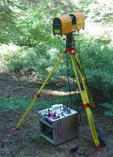
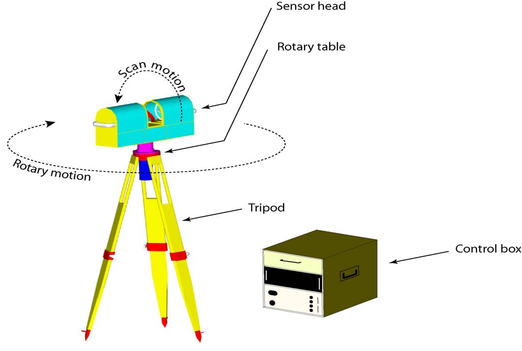
Figure 9. Echidna® ground-based lidar. Lidar pulses strike a rotating mirror at an angle of 45, providing a scan through zenith angles of 130 in a vertical circle. As the instrument rotates on its vertical axis, data from all azimuths are acquired.

Field Investigations

To test the ability of the EVI ground-based lidar to retrieve forest structural parameters, lidar scans and manual tree measurements were acquired in 2007 and 2009 at three classic New England locations: Harvard Forest, Petersham, Massachusetts; Howland Research Forest, Howland, Maine; and Bartlett Experimental Forest, Bartlett, New Hampshire. In 2008, lidar scans and manual tree measurements were acquired in the Sierra National Forest, near Clovis, California.

New England 2007 Campaign

Each plot was 100 x 100 m square (1 ha) with four 50 m x 50 m squares nested within it. True north compass readings were used to establish the grid. The compass was corrected for magnetic declination.

EVI scans were made at the center point of the square and at center points of the four 50 m x 50 m squares for a total of five scans at each site (except at Howland Research Forest Plot 2 where only three scans were made) (Table 4).

Manual measurements of trees were made in circular plots around the scan point of 20 m range (or 25 m at Harv_01 site). Each tree was numbered and identified to species. The distance from the center point to the tree was measured using a sonar or laser rangefinder. The azimuth of the tree from the center point was measured using a sighting compass (magnetic north; the compass used to measure the bearings was not corrected for magnetic declination). The tree’s diameter (DBH) at breast height (1.3 m) was measured using a diameter tape. All trees of DBH greater than 3 cm within 10 m of the plot center, and all trees of DBH greater than 10 cm beyond that distance were included. Also noted was the extent to which each tree would be visible to the EVI while scanning from the center point by tallying it as visible, partly occluded by intervening trunks or foliage, or fully occluded. In addition, 10 individual trees were selected (taken as the first tree at or beyond an azimuth increment of 36°) for measurements of the tree height, the height at which the crown began, and the crown diameter. The height of the tree was measured by a laser range finder, and the crown diameter was measured by a tape. Forest field biomass was calculated by allometric equations based on DBH measurements.

Field LAI values were measured in two ways: hemispherical canopy photograph and LAI-2000. In this study, a Nikon Coolpix 900 camera with a 180° fisheye lens pointed toward the zenith was used at a resolution of 1,391 x 1,405. All photographs were taken before sunrise or after sunset under clear sky conditions to ensure homogeneous, shadow-free illumination of the canopy and high contrast in the blue spectral region between the canopy and the sky. To properly sample the spatial variability over the plot, 13 hemispherical photographs were taken at a spacing of 10 m inside a square or 30 m on a side centered on the point. All digital photographs were collected as highest-quality JPEG images and were analyzed using HemiView software. The LAI-2000 instrument was operated in one-sensor mode, starting and ending with reference readings that are linearly scaled with time to match undercanopy readings. Transmittance is calculated from the ratio of undercanopy to open measurements for each sky sector. LAI is then retrieved by the internal software. Under canopy samples were acquired using the same sample design as hemispherical canopy photographs.

By using a"find trunks" algorithm, the investigators retrieved values of mean DBH, stem density, basal area, and above-ground woody biomass at each scan point (plot). The algorithm classifies laser returns into hard and soft targets, and works only with the hard target returns. Trunk diameter is obtained by observing the angular distance at range between the trunk’s edges. The calculation of the mean DBH of trees identified by the find trunks algorithm weights each retrieved diameter inversely by its variance, which is a function of both its size and distance. As not every tree is visible in the EVI scan because of occlusion of far trunks by near ones, the count must be adjusted for this occlusion effect. By using EVI data, the investigators used two methods to retrieve LAI from gap probability with height: single direction and multiple directions.

Sierra National Forest 2008 Campaign

Each plot was 100 x 100 m square (1 ha) in size, with 9 subplots in each plot (Figure 1). True north compass readings were used to establish the grid. The compass was corrected for magnetic declination. GPS records were made at the center of each field plot.

EVI scans were made at the center point of the square and at the corners of the central subplot .

Manual tree measurements were made in each subplot. Each tree was numbered and identified to species. The distance from the center point to the tree was measured using a sonar or laser rangefinder. The azimuth of the tree from the center point was measured using a sighting compass (magnetic north; the compass used to measure the bearings was not corrected for magnetic declination). The tree’s diameter (DBH) at breast height (1.3 m) was measured using a diameter tape. DBH and tree identification was recorded for every tree of DBH greater than 10 cm, but tree height and crown diameter were measured for a subsample (1-3) of trees in each subplot. Field LAI values were measured in three ways: hemispherical canopy photographs, TRAC, and LAI-2000. See methods for New England 2007 Campaign for details. Biomass for each stem was calculated in megagrams (Mg) using the general equations from Table 1 of Jenkins et al. 2004.

Calculation of stem biomass from Table 1 of Jenkins et al. (2004)
Allometric equation used: biomass (kg)= Exp(B0 + B1(ln(dbh (cm)))
Tree/Shrub species	B0	B1
Aspen/alder/willow	-2.2094	2.3867
Soft maple/ birch	--1.9123	2.3651
Mixed hardwood	-2.4800	2.4835
Hard maple/ oak/ beech	-2.0127	2.4342
Cedar/ larch	-2.0336	2.2592
Douglas fir	-2.2304	2.4435
True fir/ hemlock	-2.5384	2.4814
Pine	-2.5356	2.4349
Spruce	-2.0773	2.3323
Juniper/oak/ mesquite	-0.7152	1.7029
Jenkins, JC, DC Chojnacky, LS Heath and RA Birdsey. 2004. Comprehensive database of diameter-based biomass regressions for North American tree species. USDA/ Forest Service GTR-319

New England 2009 Campaign

Each plot was 50 m x 50 m with four 25 m x 25 m intensive subplots nested within it. For 3-D reconstruction, the exact Echidna® scan locations were surveyed to cm relative accuracy, in addition to GPS records. The locations of Echidna scan points in the plot were determined by triangulation (chain of triangles method) to centimeter accuracy. True north compass readings were used to establish the grid. The compass was corrected for magnetic declination.

Nine EVI scans were made in each plot: in the four corners of each plot (NW, NE, SW, and SE), in the center (C), and at N, E, S, and W locations (Figure 2).

To collect the manual tree measurements, each 50 m x 50 m plot was divided into 5 subplots (C, NW, NE, SW and SE) (Figure 3). The central subplot was a square plot, measuring 28.53 m x 28.53 m; the other subplots were isosceles right triangle plots, with 25 m right-angle side. In each subplot (C, NW, NE, SW and SE), all trees, with a diameter at breast height (DBH) equal to or larger than 10 cm, were numbered, species identified, live or dead recorded, and diameter measured. The distance from the reference point to the tree was measured using a laser rangefinder, and the bearing from the center point was determined using a sighting compass (magnetic north; the compass used to measure the bearings was not corrected for magnetic declination). The reference points were located in the center of the central subplot, and in the vertex of other subplots. Tree height, height to crown base, and crown dimensions (the longest axis and the perpendicular one) were measured on every 10th tree. The numbers of stems, with DBH smaller than 10 cm and larger or equal to 3 cm, were counted within a 10 meter distance of the reference point in each subplot (Figure 4B). Species and condition (live or dead) for the small trees was recorded. In order to register the entire plot stem map based on different reference points, some “extra” trees were selected and located to both of the central and other subplot reference points (the green points in Figure 4B).

During the 2009 campaign, the investigators revisited two sites: Harvard Forest Hemlock site (HF_HH) and Howland Forest BU Shelterwood site (HOW8), where they repeated all of the ECHIDNA® scans in the same location as 2007 (Subplot_ID C, NW, SW, and SE) and added four more scans in each site in 2009 (Subplot_ID W, E, N, and S). The GPS locations may not match to each other from 2007 to 2009 due to the GPS accuracy. For the revisited sites, the 2009 GPS locations should be the most accurate.

6. Data Access:

This data set is available through the Oak Ridge National Laboratory (ORNL) Distributed Active Archive Center (DAAC).

Data Archive:

Web Site: http://daac.ornl.gov

Contact for Data Center Access Information:

E-mail: uso@daac.ornl.gov
Telephone: +1 (865) 241-3952

7. References:

Yao, T., et al., Measuring forest structure and biomass in New England forest stands using Echidna ground-basedlidar, Remote Sensing of Environment (2011), doi:10.1016/j.rse.2010.03.019

Catovsky, S., and F.A. Bazzaz. 2000. Contributions 625 of coniferous and broad-leaved species to temperate forest carbon uptake: a bottom-up approach. Canadian Journal of Remote Sensing, 627(30): 100–111.

Cohen, W.B., T.K. Maiersperger, D.P. Turner, W.D. Ritts, and D. Pflugmacher. 2006. MODIS land cover and LAI collection 4 product quality across nine states in the western hemisphere. IEEE Transaction on Geosciences and Remote Sensing, 44(7): 1843-1856.

Jenkins, JC, DC Chojnacky, LS Heath and RA Birdsey. 2004. Comprehensive database of diameter-based biomass regressions for North American tree species. USDA/ Forest Service GTR-319.

Young HE, Ribe JH, Wainwright K (1980) Weight tables for tree and shrub species in Maine. Life Sciences and Agriculture Experiment Station, University of Maine at Orono. Miscellaneous Report 230, 84 pp.

Zhao, F., et al., Measuring effective leaf area index, foliage profile, and stand height in New England forest stands using a full-waveform ground-based lidar, Remote Sensing of Environment (2011), doi:10.1016/j.rse.2010.08.030

Additional Sources of Information:

Jupp, D.L.B., and J.L. Lovell. 2007. Airborne and ground-based lidar systems for forest measurement: background and principles. CSIRO Marine and Atmospheric Research paper, 17: 151 pp.

Jupp, D.L.B. D.S. Culvenor, J.L. Lovell, G.J. Newnham, A.H. Strahler, and C.E. Woodcock. 2008. Estimating forest LAI profiles and structural parameters using a ground-based laser called 'Echidna®'. Tree Physiology, 29: 171–181.

Magnussen, S., P. Eggermont, and V.N. LaRiccia. 1999. Recovering Tree Heights from Airborne Laser Scanner Data. Forest Science, 45(3): 407-422.

Ni-Meister, W., D.L.B. Jupp, and R. Dubayah. 2001. Modeling lidar waveforms in heterogeneous and discrete canopies. EEE Transactions on Geoscience and Remote Sensing, 39(9): 1,943-1,958.

Strahler, A. H., D.L.B. Jupp, C.E. Woodcock, C.B. Schaaf, T. Yao, F. Zhao, X. Yang, J. Lovell, D. Culvenor, G. Newnham, W. Ni-Meister, and W. Boykin-Morris. 2008. Retrieval of forest structural parameters using a ground-based lidar instrument (Echidna®). Can J. Remote Sensing, 34(Suppl. 2): S426-S440.

Yang, X., T. Yao,. A.H. Strahler, C.E. Woodcock, C.B. Schaaf, R. Myneni,. J. Liu, G.J. Newnham, D.L.B. Jupp, D.S. Culvenor, J.L. Lovell, W. Ni-Meister, S. Lee, X. Li, F. Zhao, Q. Zhang, M. Schull, M. Roman, Z. Wang, and Y. Shuai. 2008. Validation Of Improved Forest Canopy Measurements From A Ground-Based Lidar Instrument (Echidna®). Abstract. IEEE International Geoscience & Remote Sensing Symposium, Boston, Massachusetts, U.S.A.