Documentation Revision Date: 2016-11-16
Data Set Version: V1
Summary
The 65 observation sites cover nine of the 17 PFTs of the International Geosphere-Biosphere Programme (IGBP) land cover classification scheme (Loveland and Belward, 1997). MODIS Collection 5 data were used for site phenology, land surface water, enhanced vegetation index, and land surface cover type.
There are nine data files with this data set in comma-separated (*.csv) format. The files provide monthly and annual data for individual sites, all sites, and sites grouped by PFT.
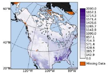
Figure 1. VPRM annual integrated respiration for 2002 provided in g C/m2/yr. Black areas are outside the study domain (Hilton et al., 2014).
Citation
Hilton, T.W., K.J. Davis, K. Keller, and N.M. Urban. 2016. NACP VPRM NEE Parameters Optimized to North American Flux Tower Sites, 2000-2006. ORNL DAAC, Oak Ridge, Tennessee, USA. http://dx.doi.org/10.3334/ORNLDAAC/1349
Table of Contents
- Data Set Overview
- Data Characteristics
- Application and Derivation
- Quality Assessment
- Data Acquisition, Materials, and Methods
- Data Access
- References
Data Set Overview
Vegetation Photosynthesis Respiration Model (VPRM) is a simple diagnostic terrestrial flux model. An overview of the model structure is provided in Section 5 of this document. VPRM calculates net ecosystem exchange (NEE) using locally observed temperature and photosynthetically active radiation (PAR) along with satellite-derived phenology and moisture. This study examined VPRM parameters optimized to 65 observed data from flux towers across North America (FLUXNET 2007 data set), locally observed temperature and PAR along with satellite-derived phenology and moisture as input data. The parameters include: β- basal rate of ecosystem respiration, α- the slope of respiration with respect to temperature, λ- light-use efficiency (LUE), and PAR0-LUE curve half-saturation. Three temporal and three spatial windows for sum of squared errors minimization were examined – in time: monthly, annual, and all available data; and, in space: individual sites, sites grouped by PFT, and all sites together.
Project: North American Carbon Program (NACP)
The North American Carbon Program (NACP) is a multidisciplinary research program designed to improve scientific understanding of North America's carbon sources and sinks and of changes in carbon stocks needed to meet societal concerns and to provide tools for decision makers.
Data Characteristics
Spatial Coverage: 65 flux tower sites across the conterminous US, Alaska, and Canada.
Spatial Resolution: Varied- These are modeled estimates using observed flux tower data and MODIS data.
Temporal Coverage: 2000 - 2006. One file provides data for 2007.
Temporal Resolution: Monthly and Annual.
Study Area (All latitudes and longitudes are given in decimal degrees)
| Site | Westernmost Longitude | Easternmost Longitude | Northernmost Latitude | Southernmost Latitude |
|---|---|---|---|---|
| North America: Conterminous US, Alaska, and Canada | -156.63 | -68.74 | 71.31999 | 28.46 |
Table 1. The 65 North American flux tower sites used to parameterize VPRM. PFTs (land cover) are taken from the International Geosphere-Biosphere Programme (IGBP) land cover classification scheme (Loveland and Belward, 1997) or investigator descriptions where available, and otherwise derived from MODIS 1 km land surface classifications (Hilton et al., 2014). In the data files with "pft" in the file names, PFT corresponds to the land cover in the table below.
| Site | Land cover (PFT) | Site name | Latitude | Longitude |
|---|---|---|---|---|
| CA-Ca1 | 1 – Evergreen Needleleaf Forest | British Columbia – Campbell River – Mature Forest Site | 49.87 | -125.534 |
| CA-ca2 | 1 – Evergreen Needleleaf Forest | British Columbia – Campbell River –Clearcut site | 49.87 | -125.29 |
| CA-ca3 | 1 – Evergreen Needleleaf Forest | British Columbia – Campbell River –Young Plantation site | 49.87 | -124.9 |
| CA-Gro | 5 – Mixed Forest | Ontario – Groundhog River-Mature Boreal Mixed Wood | 48.22 | -82.16 |
| CA-Let | 10 – Grasslands | Lethbridge | 49.71 | -112.94 |
| CA-Mer | 1 – Permanent Wetlands | Eastern Peatland – Mer Bleu | 45.1 | -75.52 |
| CA-NS2 | 1 – Evergreen Needleleaf Fores | UCI-1930 burn site | 55.91 | -98.52 |
| CA-NS3 | 1 – Evergreen Needleleaf Fores | UCI-1964 burn site | 55.91 | -98.38 |
| CA-NS4 | 1 – Evergreen Needleleaf Fores | UCI-1964 burn site | 55.91 | -98.38 |
| CA-NS5 | 1 – Evergreen Needleleaf Fores | UCI-1981 burn site | 55.86 | -98.49 |
| CA-NS6 | 1 – Evergreen Needleleaf Fores | UCI-19389 burn site | 55.92 | -98.96 |
| CA-NS7 | 1 – Evergreen Needleleaf Fores | UCI-1998 burn site | 56.64 | -99.95 |
| CA-Oas | 4 – Deciduous Broadleaf Forest | Sask – SSA Old Aspen | 53.63 | -106.2 |
| CA-Obs | 1 – Evergreen Needleleaf Forest | Sask – SSA Old Black Spruce | 53.99 | -105.12 |
| CA-Ojp | 1 – Evergreen Needleleaf Forest | Sask – SSA Old Jack Pine | 53.92 | -104.69 |
| CA-Qcu | 7 – Open Shrubland | Quebec Boreal Cutover Site | 49.27 | -74.04 |
| CA-Qfo | 1 – Evergreen Needleleaf Forest | Quebec Mature Boreal Forest Site | 49.69 | -74.34 |
| CA-SF2 | 6 – Closed Shrublands | Sask – Fire 1989 | 54.25 | -105.88 |
| CA-SF3 | 6 – Closed Shrublands | Sask – Fire 1998 | 54.09 | 106.01 |
| CA-SJ1 | 1 – Evergreen Needleleaf Forest | Sask – 1994 Harv. Jack Pine | 53.91 | -104.66 |
| CA-SJ2 | 1 – Evergreen Needleleaf Forest | Sask – 2002 Harvested Jack Pin | 53.95 | -104.65 |
| CA-WP1 | 11 – Permanent Wetlands | Western Peatland – LaBiche-Black Spruce/Larch Fen | 54.96 | -112.46 |
| US-ARM | 12 – Cropland | ARM Southern Great Plains site – Lamont – Oklahoma | 36.61 | -97.49 |
| US-Atq | 11 – Permanent Wetlands | Atqasuk – Alaska | 70.47 | -157.41 |
| US-Aud | 10 – Grasslands | Audubon Research Ranch – Arizona | 31.59 | -110.51 |
| US-Blo | 1 – Evergreen Needleleaf Forest | Blodgett Forest – California | 38.9 | -120.36 |
| US-Bn1 | 1 – Evergreen Needleleaf Forest | Delta Junction 1920 Control site | 63.92 | -145.37 |
| US-Bn2 | 4 – Deciduous Broadleaf Fores | Delta Junction 1987 Burn site | 63.92 | -145.37 |
| US-Bn3 | 7 – Open Shrublands | Delta Junction 1999 Burn site | 63.92 | -145.74 |
| US-Bo1 | 12 – Croplands | Bondville – Illinois | 40.01 | -88.29 |
| US-Bo2 | 12 – Croplands | Bondville – Illinois (companion site) | 40.01 | -88.29 |
| US-Brw | 11 – Permanent Wetlands | Barrow – Alaska | 71.32 | -156.63 |
| US-CaV | 10 – Grasslands | Canaan Valley – West Virginia | 36.06 | -79.42 |
| US-Dk1 | 10 – Grasslands | Duke Forest-open field – North Carolina | 35.97 | -79.09 |
| US-Dk2 | 4 – Deciduous Broadleaf Forest | Duke Forest-hardwoods – North Carolina | 35.97 | -79.1 |
| US-Dk3 | 1 – Evergreen Needleleaf Fores | Duke Forest – loblolly pine – North Carolina | 35.98 | -79.09 |
| US-FPe | 10 – Grasslands | Fort Peck – Montana | 48.31 | -105.1 |
| US-Goo | 10 – Grasslands | Goodwin Creek- Mississippi | 34.25 | -89.97 |
| US-Ha1 | 4 – Deciduous Broadleaf Forest | Harvard Forest EMS Tower – Massachusetts (HFR1 | 42.54 | -72.17 |
| US-Ha2 | 1 – Evergreen Needleleaf Forest | Harvard Forest Hemlock Site – Massachusetts | 42.54 | -72.17 |
| US-Ho1 | 1 – Evergreen Needleleaf Forest | Howland Forest (main tower) – Maine | 45.2 | -68.74 |
| US-Ho2 | 1 – Evergreen Needleleaf Forest | Howland Forest (west tower) – Maine | 45.21 | -68.75 |
| US-KS1 | 1 – Evergreen Needleleaf Forest | Florida-Kennedy Space Center (slash pine) | 28.46 | -80.67 |
| US-KS2 | 6 – Closed Shrublands | Florida-Kennedy Space Center (scrub oak) | 28.61 | -80.67 |
| US-Los | 6 – Closed Shrublands | Lost Creek – Wisconsin | 46.08 | -89.98 |
| US-Me2 | 1 – Evergreen Needleleaf Forest | Metolius-intermediate aged ponderosa pine – Oregon | 44.55 | -121.56 |
| US-Me4 | 1 – Evergreen Needleleaf Forest | Metolius-old aged ponderosa pine – Oregon | 44.5 | -121.62 |
| US-MMS | 4 – Deciduous Broadleaf Forest | Morgan Monroe State Forest – Indiana | 39.32 | -86.41 |
| US-MOz | 4 – Deciduous Broadleaf Forest | Missouri Ozark Site | 38.74 | -92.2 |
| US-Ne1 | 12 – Croplands | Mead – irrigated continuous maize site – Nebraska | 41.1 | -96.29 |
| US-Ne2 | 12 – Croplands | Mead – irrigated maize-soybean rotation site – Nebraska | 41.1 | -96.28 |
| US-Ne3 | 12 – Croplands | Mead – rainfed maize-soybean rotation site – Nebraska | 41.18 | -96.44 |
| US-NR1 | 1 – Evergreen Needleleaf Forest | Niwot Ridge Forest – Colorado (LTER NWT1) | 40.03 | -105.55 |
| US-PFa | 5 – Mixed Fores | Park Falls/WLEF – Wisconsin | 45.95 | -90.27 |
| US-SO2 | 6 – Closed Shrublands | Sky Oaks – Old Stand – California | 33.37 | -116.62 |
| US-SO3 | 6 – Closed Shrublands | Sky Oaks – Young Stand – California | 33.38 | -116.62 |
| US-SO4 | 6 – Closed Shrublands | Sky Oaks – California | 33.37 | -116.62 |
| US-SP1 | 1 – Evergreen Needleleaf Fores | Slashpine-Austin Cary – 65 yr nat regen-FL | 29.74 | -82.22 |
| US-SP2 | 1 – Evergreen Needleleaf Fores | Slashpine-Mize-clearcut-3 yr-regen-FL | 29.76 | -82.24 |
| US-SP3 | 1 – Evergreen Needleleaf Fores | Slashpine-Donaldson-mid-rot – 12 yr-FL | 29.75 | -82.16 |
| US-Syv | 5 – Mixed Forest | Sylvania Wilderness Area – Michigan | 46.24 | -89.35 |
| US-Ton | 8 – Woody Savannas | Tonzi Ranch – California | 38.43 | -120.97 |
| US-UMB | 4 – Deciduous Broadleaf Forest | Univ. of Mich. Biological Station – Michigan | 45.56 | -84.71 |
| US-Var | 10 – Grasslands | Vaira Ranch – Ione – California | 38.41 | -120.95 |
| US-WCr | 4 – Deciduous Broadleaf Forest | Willow Creek – Wisconsin | 45.81 | -90.08 |
Data File Information
There are nine data files in comma-separated (.csv) format with this data set. The files provide VPRM parameter values optimized to 65 flux tower sites across North America. The data are for the time period 2000-2007. Not all files include the entire period. Only one file includes data for 2007. There are no missing values.
Table 2. File names and descriptions
| File name | Description | Number of observations in each file |
|---|---|---|
| VPRM_parameters_all_sites_all_data.csv | This file provides parameter values for all years combined and site (site = "all") | 1 |
| VPRM_parameters_all_sites_annual_data.csv | This file provides yearly data for the years 2000 – 2007 for each of the four parameters and site (site = "all") | 8 |
| VPRM_parameters_all_sites_monthly_data.csv | This file provides parameter values for each month for each year for 2000 – 2006 and site (site = "all") | 85 |
|
VPRM_parameters_individual_sites_all_data.csv
|
This file provides yearly parameter values for each of the 65 sites and “site”, which is the Fluxnet site ID. Note that there is not data for each year for each site. There is one year of data for each site. The data are for the period 2000 – 2004 where data are provided for some sites for the year 2000 and for other sites for 2001, etc. | 65 |
| VPRM_parameters_individual_sites_annual_data.csv | This file provides parameter values for each of the 65 sites by year for the period 2000 – 2006. Note that data are not provided for every year for each site. This file also includes “site” which is the Fluxnet site ID. | 286 |
| VPRM_parameters_individual_sites_monthly_data.csv | This file provides parameter values for each of the 65 sites for each month for the years 2000 – 2006. Note that data are not provided for every year for each site. This file also includes “site” which is the Fluxnet site ID. | 3,432 |
| VPRM_parameters_pft_sites_all_data.csv | This file provides parameter values by nine PFT classes for the year 2000 only. | 9 |
| VPRM_parameters_pft_sites_annual_data.csv | This file provides parameter values by nine PFT classes for each year for 2000 – 2006 | 61 |
| VPRM_parameters_pft_sites_monthly_data.csv | This file provides parameter values by nine PFT classes for each month for each year for 2000 – 2006. | 732 |
Table 3. Parameters in the data files
| Site | This is provided in the files named VPRM_parameters_individual_sites__. This is the FLUXNETsite ID. It is also provided in the files named VPRM_parameter_values_all_sites, and the value is "all" |
| PFT | This is only in files named VPRM_parameters_pft_sites__. This is the land cover classification number as provided by Hilton et al., 2013. Refer to Table 1. |
| tstamp | Time stamp. Refers to the year or date of the provided data, in yyyy or yyyy-mm-dd. |
| lambda | Maximum light use efficiency |
| alpha | Slope of respiration with respect to temperature |
| beta | Basal respiration rate |
| PAR_0 | LUE half-saturation value (PAR0 in the model) |
Application and Derivation
Our findings are relevant to both land surface model upscaling as well as atmospheric inversion studies.
Quality Assessment
The structural simplicity of VPRM allows parameter estimations to be conducted that use many thousands of model evaluations. However, caution is advised against attempting site-specific ecological interpretation of short-term fluctuations in VPRM parameter values, fluxes, and residuals.
Data Acquisition, Materials, and Methods
VPRM calculates net ecosystem exchange (NEE) using locally observed temperature and photosynthetically active radiation (PAR) along with satellite-derived phenology and moisture. Temperature and PAR can come from site-level observations when modeling a point. VPRM does not consider driver data or flux results from previous time steps.
VPRM data inputs
Observed input data were from 65 flux towers across North America. These data are part of the 2007 FLUXNET Synthesis data set (http://www.fluxdata.org). For each site, this data set contains CO2 flux, air temperature, and PAR observations at 30 min intervals, as well as many other quantities not needed for VPRM. The 65 observation sites cover nine of the 17 PFTs of the International Geosphere-Biosphere Programme (IGBP) land cover classification scheme (Loveland and Belward, 1997): evergreen needleleaf forest (27 sites), deciduous broadleaf forest (8 sites), mixed forest (3 sites), closed shrublands (7 sites), open shrublands (2 sites), woody savannas (1 site), grasslands (7 sites), permanent wetlands (4 sites), and croplands (6 sites).
MODIS Collection 5 data were used for site phenology, land surface water, enhanced vegetation index, and land surface cover type:
- Site phenology is from data set M*D12Q2 (Strahler et al., 1999a)
- Reflectances are from data set M*D43A4 (Strahler et al., 1999b)
- Vegetation indices are from data set M*D13A2 (Huete et al., 2002, and 1999)
- IGBP land surface cover types are from data set M*D12Q1 (Loveland and Belward, 1997; Strahler et al.,1999a).
The “*” in M*D is either “O”, representing the data from the Terra satellite, or “Y” representing the data from the Aqua satellite. Only MODIS data of “best” quality, as indicated by each MODIS product’s associated quality assurance flags were considered (Hilton et al., 2013).
The time period examined was 2000 to 2006, bounded in 2000 by the MODIS instrument launch and in 2006 by eddy covariance flux availability.
The VPRM model
VPRM is a simple diagnostic terrestrial flux model. VPRM models net ecosystem exchange (NEE) as the sum of a photosynthetic component (gross ecosystem exchange, GEE) and an ecosystem respiration component. An overview of the model structure followed by the definitions of the four parameters studied and included with this data set are provided below (refer to Hilton et al., 2013 and 2014).
GEE is modeled via the equation:
(1) GEE = λ·Tscale·Pscale·Wscale·EVI·1/1+PAR/PAR0·PAR
PAR is observed photosynthetically active radiation and EVI is the satellite-derived enhanced vegetation index (Huete et al., 2002). PAR0 and λ are user-supplied parameters.
Pscale, Wscale, and Tscale are dimensionless scaling terms. They each take values between 0.0 and 1.0 and are defined as follows:
Pscale is satellite derived and describes the impacts of leaf expansion and senescence on canopy-scale photosynthesis. Pscale is defined as 0.0 outside of the growing season, 1.0 during growing season peak greenness, and is a linear function of the satellite-derived land surface water index (LSWI) (Xiao et al., 2004) during leaf expansion and senescence.
(2) Pscale = 1+LSWI/2
Wscale is satellite derived and describes canopy moisture, and is defined as:
(3) Wscale = 1+LSWI/1+LSWImax
with LSWImax the growing-season maximum LSWI value. The value of the third dimensionless scaling term Tscale is taken from literature and describes the relationship between photosynthesis and temperature.
Tscale is defined as:
(4) Tscale = (T-Tmin) (T-Tmax)/ (T-Tmin) (T-Tmax) – (T-Topt)2
Pscale, Wscale, and Tscale by definition, vary in both time and space (Mahadevan et al., 2008). Respiration (R) is modeled as a linear function of observed surface air temperature (T):
(5) R = α·T+β
with user-supplied parameters α and β. NEE is the difference between the photosynthetic flux and the respiration flux:
(6) NEE = R - GEE
Four estimated parameters:
Within equations (1), (5), and (6), are the four estimated parameters provided in this data set:
- λ governs the slope of the light-response curve (the relationship between photosynthetic CO2 flux and PAR)
- α defines the slope of the respiration response to temperature
- PAR0 defines a half saturation value for photosynthesis. That is, it specifies a PAR value at which further increases in PAR no longer enhance photosynthesis, as other limiting factors become dominant.
- β thus specifies a minimal level of respiration that occurs regardless of air temperature.
The source code used to estimate these parameter values is available at https://github.com/Timothy-W-Hilton/VPRMLandSfcModel.
VPRM NEE parameters
Model residuals are the combined effects of flux observation errors, model structural error, and natural variability uncaptured by the flux model. The goal was to have VPRM parameters that caused VPRM NEE to closely match observed NEE (Hilton et al., 2013).
NEE varies on a number of different time scales (e.g.,daily, annual) and space scales (e.g., local land use and PFT heterogeneity, larger regions that experience similar climate patterns). An ideal land surface model parameter estimation method would allow parameter values to vary at space and time scales matching the ecological variations in NEE. Optimizing parameter values in short time intervals and small spatial windows would run the risk of overfitting as well as incur unnecessary computational cost. In this study, three temporal and three spatial windows for the sum of squared errors (SSE; we define VPRM residuals as NEEVPRM minus NEEobserved) minimization were examined:
- in time: monthly, annual, and all available data
- in space: individual sites, sites grouped by PFT, and all sites together.
This approach resulted in nine different parameter sets.
To search for parameter values that minimized SSE, differential evolution (DE) (Price et al., 2006) was used. DE is a genetic optimization algorithm that is both fast and more reliable in identifying a global optimum compared to gradient-based minimization algorithms. The DEoptim package (Ardia and Mullen, 2009) for the R language and platform for statistical computing (R Development Core Team, 2007) was used.
The Markov chain Monte Carlo (MCMC) optimization approach offers the advantage of delivering probability density functions (PDFs), and thus parameter uncertainties, rather than the single optimal value estimates provided by DE. Because of the substantially increased computational expense and the lack of a statistically robust residual likelihood function, DE was chosen to obtain the point estimates provided (Hilton et al., 2013).
VPRM NEE residual spatial structure
Semivariograms were used to evaluate residual spatial structure. Because VPRM NEE residuals are simply the difference between NEEobs and NEEVPRM, the spatial behaviors of these three quantities are interrelated.
For additional information, please refer to Hilton et al. 2013 and 2014.
Data Access
These data are available through the Oak Ridge National Laboratory (ORNL) Distributed Active Archive Center (DAAC).
NACP VPRM NEE Parameters Optimized to North American Flux Tower Sites, 2000-2006
Contact for Data Center Access Information:
- E-mail: uso@daac.ornl.gov
- Telephone: +1 (865) 241-3952
References
Ardia, D. and K. Mullen. 2009. DEoptim: Differential Evolution Optimization in R, R package version 2.0-1, http://CRAN.R-project. org/package=DEoptim (last access: 1 June 2012), 2009.
Hilton, T.W., K. J. Davis, and K. Keller. 2014. Evaluating terrestrial CO2 flux diagnoses and uncertainties from a simple land surface model and its residuals, Biogeosciences, 11, 217-235, doi:10.5194/bg-11-217-2014.
Hilton, T.W., K. J. Davis, K. Keller, and N.M. Urban. 2013. Improving North American terrestrial CO2 flux diagnosis using spatial structure in land surface model residuals, Biogeosciences, 10,4607–4625, doi:10.5194/bg-10-4607-2013.
Huete, A., K. Didan, T. Miura, E. Rodriguez, X. Gao, and L. Ferreira, L. 2002. Overview of the radiometric and biophysical performance of the MODIS vegetation indices, Remote Sens. Environ.,83, 195–213, 2002.
Huete, A., C. Justice, and W. van Leeuwen. 1999. MODIS vegetation index (MOD 13) algorithm theoretical basis document, Version 3, available at: http://modis.gsfc.nasa.gov/data/atbd/atbd_mod13.pdf (last access: 1 June 2012.
Loveland, T. and A. Belward. 1997. The IGBP-DIS global 1km land cover data set, DISCover: first results, Int. J. Remote Sens., 18, 3289–3295, 1997.
Mahadevan, P., S. Wofsy, D. Matross, X. Xiao, A. Dunn, J. Lin, C. Gerbig, J. Munger, V. Chow, and E. Gottlieb. 2008. A Satellite-Based Biosphere Parameterization for Net Ecosystem CO2 Exchange: Vegetation Photosynthesis and Respiration Model (VPRM), Global Biogeochem. Cy., 22, GB2005, doi:10.1029/2006GB002735
Price, K., R. Storn, R., and J. Lampinen. 2006. Differential Evolution – A Practical Approach to Global Optimization, Springer, Berlin, Germany, ISBN number: 3540209506
Strahler, A., D. Muchoney, J. Borak, M. Friedl, S. Gopal, E. Lambin, and A. Moody. 1999a. MODIS Land Cover Product Algorithm Theoretical Basis Document (ATBD) MODIS Land Cover and Land-Cover Change, USGS, NASA, http://modis.gsfc.nasa.gov/data/atbd/atbd_mod12.pdf , (last accessed: 4 June 2012).
Strahler, A. H., W. Lucht, C.B. Schaaf, T. Tsang, F. Gao, X. Li, J.P. Muller, P. Lewis, and M. Barnsley. 1999b. MODIS BRDF/albedo product: algorithm theoretical basis document version 5.0, http://modis.gsfc.nasa.gov/data/atbd/atbd_mod09.pdf (last accessed 4 June 2012.
Xiao, X., Q. Zhang, B. Braswell, S. Urbanski, S. Boles, S. Wofsy, B. Moore, and D. Ojima. 2004. Modeling gross primary production of temperate deciduous broadleaf forest using satellite images and climate data, Remote Sens. Environ., 91, 256–270.