Documentation Revision Date: 2022-12-29
Dataset Version: 1
Summary
There are four compressed (*.zip) files with this dataset that provide model code, GIS input files, spectral data input files, and model output files.The model code is in Python; input data are in comma-separated values (CSV), GeoTIFF and shapefile formats, and model output files are in GeoTIFF and binary NumPy formats.
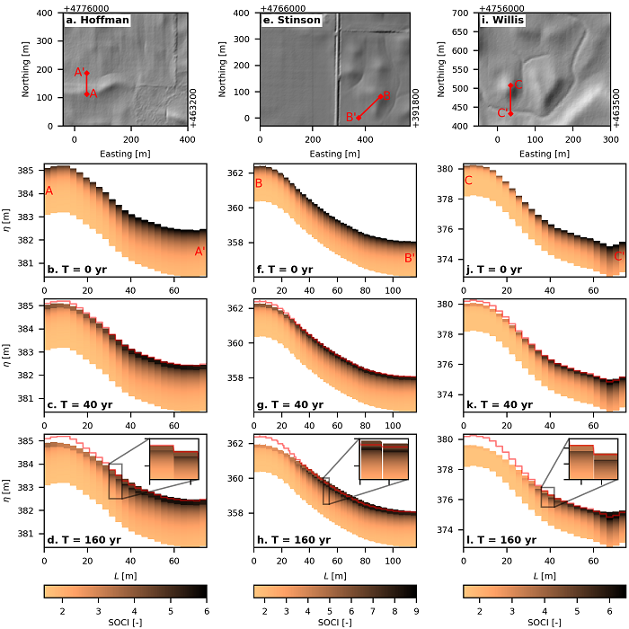
Figure 1. Hillslope transects at three sites showing redistribution of soil organic carbon (SOC) simulated over 160 years in Iowa. Sites (columns): Hoffman, Stinson, and Willis. Upper row shows hillshade maps illustrating topography at each site. Red lines show location of transects proceeding from upslope to downslope (e.g., A to A'). Lower three rows illustrate pattern of SOC along the transect distance (L) at soil depths at beginning of simulation (0 y), after 40 y, and at end of simulation (160 y). Red lines indicate the initial surface elevation at beginning of simulation. Insets highlight cases where soil with low SOC blankets soil with higher SOC.
Citation
Kwang, J.S., E.A. Thaler, and I.J. Larsen. 2022. Topographic and Soil Carbon Reconstructions in Agricultural Fields, Iowa. ORNL DAAC, Oak Ridge, Tennessee, USA. https://doi.org/10.3334/ORNLDAAC/1944
Table of Contents
- Dataset Overview
- Data Characteristics
- Application and Derivation
- Quality Assessment
- Data Acquisition, Materials, and Methods
- Data Access
- References
Dataset Overview
This dataset contains model predictions of soil erosion and soil organic carbon (SOC) redistribution caused by agricultural practices, such as tillage erosion. Soil erosion diminishes agricultural productivity by driving the loss of SOC. This model addresses a growing need to predict soil organic carbon transport, loss, and deposition. The model was applied to three sites containing paired prairie grassland and field plots in Iowa, and predicts SOC redistribution between 1859 to 2019. The model was developed by incorporating a SOC mixing model with a landscape evolution model that simulates tillage erosion.
Project: North American Carbon Program (NACP)
The North American Carbon Program (NACP) is a multidisciplinary research program designed to improve understanding of North America's carbon sources, sinks, and stocks. The central objective is to measure and understand the sources and sinks of Carbon Dioxide (CO2), Methane (CH4), and Carbon Monoxide (CO) in North America and adjacent oceans. The NACP is supported by a number of different federal agencies.
Related Publication:
Kwang, J.S., E.A. Thaler, B.J. Quirk, C.L. Quarrier, and I.J. Larsen. 2022. A landscape evolution modeling approach for predicting three-dimensional soil organic carbon redistribution in agricultural landscapes. Journal of Geophysical Research: Biogeosciences, 127:e2021JG006616. https://doi.org/10.1029/2021JG006616
Acknowledegment: This project was funded by NASA grant 80NSSCK0747.
Data Characteristics
Spatial Coverage: Three study sites in northern Iowa, U.S.
Spatial Resolution: 3-m raster cells and point locations
Temporal coverage: 1859-08-01 to 2019-08-01 for modeling; 2017-04-07 to 2020-05-15 for imagery
Temporal resolution: Decadal estimates
Study Area: All latitudes and longitudes given in decimal degrees
| Site | Westernmost Longitude | Easternmost Longitude | Northernmost Latitude | Southernmost Latitude |
|---|---|---|---|---|
| northern Iowa | -94.3345 | -94.3211 | 43.0457 | 43.0385 |
Data File Information
This dataset includes four .zip files: model_code.zip, GIS_data_input.zip, spectral_data_input.zip, and model_results.zip. The files provide model code, GIS input files, spectral data input files, and model output files. The model code is in Python; input data are in comma-separated values (CSV), GeoTIFF and shapefile formats, and model output files are in GeoTIFF and binary NumPy formats. Tables 1-4 describe the folder structure of the .zip files (files, folders and subfolders). Table 5 provides a data dictionary for the variables in all files.
Data File Details
- The no data value for all input files is -9999.
- GeoTIFFs and other raster files are projected in UTM, zone 15, NAD83 datum (EPSG 26915).
- Raster cells are 3 m x 3 m.
Table 1. Files in model_code.zip. The results folder in this archive has three subfolders, one for each site.
| Folder name | File name | Format | Description |
|---|---|---|---|
| . | run_example.bat | text | Example batch file for running code |
| . | SOC_LEM.py | Python | Source code that models transport of soil organic carbon |
| drivers | Python | Driver files in Python | |
| input | text | Three model input files for each site: DEM (meters), soil organic carbon index (unitless) and NDVI (unitless). | |
| results | This folder contains example input and output files organized by a subfolder for each of three sites: "hoffman", "stinson", and "willis". Each subfolder holds model input files and output files with the names listed below | ||
| example_aaaa.py | Python | Driver file to generate the results. aaaa = site name: "hoffman", "stinson", or "willis" |
|
| padded_aaaa__bbbb.txt | text | Input rasters as ASCII grids. bbbb= variables: "DEM", "NDVI", "SOCI", and "depressions" (topographic depressions) | |
| 3D_SOC_000XXXyrs.npy | NumPy binary (.npy) | 3-dimensional SOCI file where indices are the following [longitude, latitude, depth]. XXX = simulation timestep (0 to 200 y) | |
| 3D_surface_XXXXXXyrs.nyp | NumPy binary (.npy) | 2-dimensional elevation file where indices are the following (easting, northing) | |
| elevation.npy | NumPy binary (.npy) | Evolution data for surface elevation (m) with indices (time, easting, northing) | |
| SOCI.npy | NumPy binary (.npy) | Evolution data for soil organic matter index with indices (time, easting, northing) | |
| utilities | pad_rasters.py | Python | Supporting code |
Table 2. Files in GIS_data_input.zip.
| Folder | File.name | Format | Description |
|---|---|---|---|
| DEM | aaaa_DEM.tif | GeoTIFF | Digital elevation model (m). aaaa = site name |
| NDVI | aaaa_NDVI.tif | GeoTIFF | Normalized difference vegetation index raster |
| SOCI | aaaa_SOCI.tif | GeoTIFF | Soil organic carbon index (unitless) raster (Thaler et al., 2019) |
| shapefiles | core_locations.shp | shapefile | Multipoint shapefile with locations of soil cores |
| surface_aaaa.shp | shapefile | Multipoint shapefile with locations of surface samples |
Table 3. Files in spectral_data_input.zip.
| File.name | Format | Description |
|---|---|---|
| aaaa_19_cccc_dddd.csv | CSV | Soil organic carbon index (SOCI). aaaa = site name. cccc = "p12c" or "p137cs". dddd = name of soil core location. |
| surface_samples_soci.csv | CSV | Surface sample names and their measured SOCI values |
Table 4. Files in model_results.zip. This zip file includes folders at three hierarchical levels in the three subfolders named hoffman, stinson, and willis.
| Folder | Primary subfolder (one for each site) | Secondary subfolder (simulation experiments) | Description |
|---|---|---|---|
| basecase These simulations use the base values of surface concentration of SOC (variable B), rate of SOC decay by depth (variable C), and plow depth (Lp) |
hoffman | inital_topography=modern_topography | These simulations hold topography constant |
| inital_topography=modern_topography+T_diffusion_eeee | These simulations vary topographic change due to erosion and deposition. eeee = a T_diffusion value ranging from 10 to 200 (see parameter D, which controls rate of erosion and deposition, described in Table 5 and Section 5) (20 folders) |
||
| stinson | Simulations for the stinson site with the same folder structure as hoffman folder. | ||
| willis | Simulations for the willis site with the same folder structure as hoffman folder. | ||
| B_sensitivity These simulations use the base values of variables C and Lp but vary values of surface SOCI (variable B) |
hoffman | +SE_B_initial_topography=modern_topography | The value of B is increased one standard error of B with constant topography |
| -SE_B_initial_topography=modern_topography | The value of B is decreased one standard error of B with constant topography | ||
| +SE_B_initial_topography=modern_topography+T_diffusion_eeee | The value of B is increased one standard error of B, and rate of topographic change values with T_diffusion parameter (eeee) from 10 to 200 (20 folders) | ||
| -SE_B_initial_topography=modern_topography+T_diffusion_eeee | The value of B is decreased one standard error of B, and rate of topographic change values with T_diffusion parameter (eeee) from 10 to 200 (20 folders) | ||
| stinson | Simulations for the stinson site with the same folder structure as hoffman folder. | ||
| willis | Simulations for the willis site with the same folder structure as hoffman folder. | ||
| C_sensitivity These simulations use the base values of variables B and Lp but vary values of rate of SOC decay by depth (variable C) |
hoffman | +SE_C_initial_topography=modern_topography | The value of C is increased one standard error of C with constant topography. This standard error is associated with a linear regression model between fitted values of C to soil cores and the topographic curvature of the surface |
| -SE_C_initial_topography=modern_topography | The value of C is decreased one standard error of C with constant topography | ||
| +SE_C_initial_topography=modern_topography+T_diffusion_eeee | The value of C is increased one standard error of C, and rate of topographic change varies with T_diffusion parameter (eeee) from 10 to 200 (20 folders) | ||
| -SE_C_initial_topography=modern_topography+T_diffusion_eeee | The value of C is decreased one standard error of C, and rate of topographic change varies with T_diffusion parameter (eeee) from 10 to 200 (20 folders) | ||
| stinson | Simulations for the stinson site with the same folder structure as hoffman folder. | ||
| willis | Simulations for the willis site with the same folder structure as hoffman folder. | ||
| Lp_sensitivity These simulations use the base values of variables B and C but vary values of plow depth (variable Lp) |
hoffman | +SE_Lp_initial_topography=modern_topography | The value of Lp is increased by one standard error of Lp with constant topography. This standard error is associated with the standard deviation of Rapid Carbon Assessment soil core measurements of the A-horizon plow layer. Note that the model files sometimes refer to the plow layer depth, Lp, as La |
| -SE_Lp_initial_topography=modern_topography | The value of Lp is decreased by one standard error of Lp with constant topography | ||
| +SE_Lp_initial_topography=modern_topography+T_diffusion_eeee | The value of Lp is increased by one standard error of Lp, and rate of topographic change varies with T_diffusion parameter (eeee) from 10 to 200. 20 folders. | ||
| -SE_Lp_initial_topography=modern_topography+T_diffusion_eeee | The value of Lp is decreased by one standard error of Lp, and rate of topographic change varies with T_diffusion parameter (eeee) from 10 to 200 (20 folders) | ||
| stinson | Simulations for the stinson site with the same folder structure as hoffman folder | ||
| willis | Simulations for the willis site with the same folder structure as hoffman folder | ||
| sheetflow These simulations vary sheetflow erosion using the base values of B, C, and Lp. The parameter K describes how erodible the soil is to water erosion (m0.5 y-1). Five values of K are 0.0, 1E-3, 1E-4, 5E-3, 5E-4 are used for all sites |
hoffman | hoffman_D=0.25_K=ffff | Simulations for the hoffman sites where the value of hillslope diffusion coefficient (D) is constant at 0.25 (five folders) |
| stinson | stinson_D=0.59_K=ffff | Simulations for stinson site where D is constant at 0.59 (five folders) | |
| willis | willis_D=0.19_K=ffff | Simulations for willis site where D is constant at 0.19 (five folders) | |
| Files in secondary subfolders | |||
| File names | File format | Description | |
| driver.py | Python | Driver file for simulation | |
| elevation_dim_T_ffff.tif | GeoTIFF | Elevation raster. ffff = simulation time step | |
| soci_dim_T_ffff.tif | GeoTIFF | Soil organic carbon index raster. ffff = simulation time step | |
Table 5. Data dictionary covering all files.
| Variable | Units | Description |
|---|---|---|
| SOCI | Soil organic carbon index = (blue reflectance)/(red reflectance x green reflectance) (Thaler et al., 2019) | |
| A | Minimum SOCI at greatest depth. Set at 1.60 | |
| B | Surface SOCI minus A | |
| C | m-1 | Rate of decay in SOCI with depth from surface |
| D | m2 y-1 | Hillslope diffusion coefficient related to tillage erosion. Same as "T_diffusion" parameter listed in folder names in Table 4 |
| K | m0.5 y-1 | Soil erodibility related to sheetflow erosion |
| elevation | m | Surface elevation |
| x | m | UTM easting coordinate, zone 15 N, NAD83 datum, EPSG 26915 |
| y | m | UTM northing coordinate, zone 15 N, NAD83 datum, EPSG 26915 |
| z | m | Depth coordinate referenced to surface |
Application and Derivation
Soil erosion diminishes agricultural productivity by driving the loss of soil organic carbon. This model addresses a growing need to understand and predict soil organic carbon transport, loss, and deposition. The ability to predict SOC redistribution is important for guiding sustainable agricultural practices and determining the influence of soil erosion on the carbon cycle.
Quality Assessment
To understand the uncertainty of model predictions, three key input parameters in our model were varied in the set simulations. Two of the inputs are linear regression models that relate topographic curvature with SOC properties of soil cores. Parameter estimates from the regression models were varied by one standard error or one standard deviation to propagate uncertainty in model predictions. The model produced spatial patterns of soil loss comparable to those observed in satellite images. See Kwang et al. (2022) for details.
Data Acquisition, Materials, and Methods
This landscape evolution model couples soil mixing and transport to predict soil loss and spatial pattern of soil organic carbon (SOC) within agricultural fields. This reduced complexity numerical model requires two physical parameters: a plow mixing depth (Lp) and a hillslope diffusion coefficient (D), which controls soil erosion and deposition. Using topography as an input, the model predicts spatial patterns of surficial SOC concentrations and complex three-dimensional SOC pedostratigraphy. Soil cores from native prairies were used to determine initial SOC-depth relationships, which served as the initial conditions in the simulations. The spatial pattern of remote sensing-derived SOC in adjacent agricultural fields was used to evaluate model predictions. The model reproduces spatial patterns of soil loss comparable to those observed in satellite images.
There were three study sites in northern Iowa (hoffman, stinson, and willis). At each one, an agricultural field was paired with an adjacent uncultivated prairie (Figure 2).
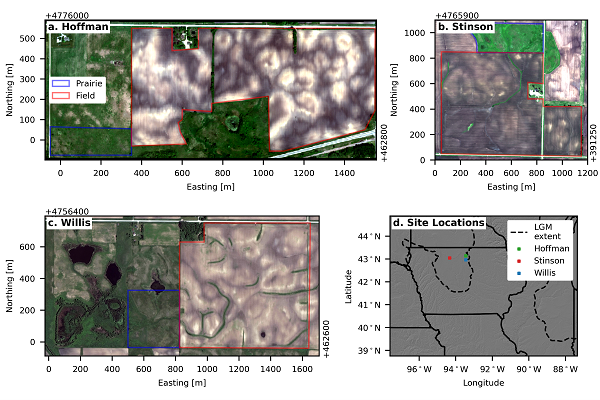
Figure 2. Satellite imagery of the (a) Hoffman (captured on 5 May 2016 with GeoEye-1), (b) Stinson (captured on 7 June 2014 with GeoEye-1), and (c) Willis sites (captured on 3 June 2020 with Worldview-2) and (d) a map of their locations in northern Iowa. Each field site contains a paired native tallgrass prairie (outlined in blue) and agricultural field (outlined in red). The dashed lines in (d) show the maximum ice sheet extent during the Last Glacial Maximum (LGM) (Dalton et al., 2020).
Input variables
Soil organic carbon index (SOCI): To estimate the initial conditions of soil organic carbon, SOCI values were measured from 33 field collected soil cores from the prairies at each study site. Spectral signatures were measured on dried soil cores in the laboratory (SOCIlab) using a ASD Fieldspec spectroradiometer with a Muglight attachment. Reflectance values for red (Nr, 590–670 nm), green (Ng, 500–590 nm), and blue bands (Nb, 455-415 nm) were normalized, and SOCI was calculated using the method of Thaler et al. (2019):
SOCIlab = Nb / (Nr x Ng)
At each site, a map of present-day surficial SOCI was produced using 3-m resolution PlanetScope satellite imagery (2017 - 2020) of the agricultural field taken in the spring prior to planting when bare soil in each field was exposed by prior tillage, and crop residue cover was minimal. The same method was used to measure SOCIsatellite, using satellite reflectance values, and a regression model was used to convert the SOCIsatellite estimates to SOCIlab values, which were used in the model.
SOCI varied by depth from soil surface, and this variation was modeled with regression equation:
SOCI(d) = A + B*e-Cd, where
A = minimum SOCI value associated with B-horizon (set to 1.6), A + B = SOCI at soil surface, C is a decay constant, and d is depth from surface. C controls the initial carbon stock in the soil profile.
Erosion and deposition (D): Changes in surface topography were simulated with a hillslope diffusion model:
dn/dt = D*(topographic curvature)*n, where
n = surface elevation and D is a mass-dependent diffusion coefficient estimated from soil bulk density. Curvature maps were developed from a LiDAR-derived DEM (State of Iowa, 2020). In this model, soil is removed from convex surfaces (ridges, negative curvature) and deposited in concave surfaces (hollows, positive curvature) (Figure 1). Soil movement depended on the topographic gradient (slope). The modern topographic surface was used for the initial condition because the topography of 150 years prior was unknown. To account for this uncertainty, simulations were conducted with varied values of D.
User note: D is the "T_diffusion" parameter included in folder names in the model_results.zip archive (Table 4).
Plow depth (Lp): By mixing the soil, plowing homogenizes SOCI from the surface to depth of plowing (Lp). SOCI is uniform from surface to Lp, and SOCI is redistributed by erosion or deposition. When the landscape is eroding, the plow layer lowers into the soil profile to unearth carbon stored in the substrate. In this case, the flux of carbon added to the plow layer is equal to the product of the rate of erosion and the concentration of carbon in soils below Lp. Where deposition occurs, a portion of the plow layer is buried and exits the plow layer to become substrate (Figure 1).
Simulation experiments and sensitivity analysis: A series of simulations were run that varied the values of B, C, Lp, and D. Values of B and C were varied by +/- one standard error from the regression analysis described above. Plow depth (Lp) was varied by +/- 5 cm. Simulation results revealed that the model is most sensitive to uncertainty in B, the initial surface value of SOCI. Moreover, valid values of D ranged from 0.10 to 0.43 m-2 y-1 and had to be adjusted to improve model fit when B and C were altered.
See Kwang et al. (2022) for a detailed description of this model and the modeling results.
Data Access
These data are available through the Oak Ridge National Laboratory (ORNL) Distributed Active Archive Center (DAAC).
Topographic and Soil Carbon Reconstructions in Agricultural Fields, Iowa
Contact for Data Center Access Information:
- E-mail: uso@daac.ornl.gov
- Telephone: +1 (865) 241-3952
References
Dalton, A.S., M. Margold, C.R. Stokes, L. Tarasov, A.S. Dyke, R.S., Adams, S. Allard, H.E. Arends, N. Atkinson, J.W. Attig, P.J. Barnett, R.L. Barnett, M. Batterson, P. Bernatchez, H.W. Borns, A. Breckenridge, J.P. Briner, E. Brouard, J.E. Campbell, A.E. Carlson, J.J. Clague, B.B. Curry, R.-A. Daigneault, H. Dubé-Loubert, D.J. Easterbrook, D.A. Franzi, H.G. Friedrich, S. Funder, M.S. Gauthier, A.S. Gowan, K.L. Harris, B. Hétu, T.S. Hooyer, C.E. Jennings, M.D. Johnson, A.E. Kehew, S.E. Kelley, D.Kerr, E.L. King, K.K. Kjeldsen, A.R. Knaeble, P. Lajeunesse, T.R. Lakeman, M. Lamothe, P. Larson, M. Lavoie, H. M. Loope, T.V. Lowell, B.A. Lusardi, L. Manz, I. McMartin, F.C. Nixon, S. Occhietti, M.A. Parkhill, D.J.W. Piper, A.G. Pronk, P.J.H. Richard, J.C. Ridge, M. Ross, M. Roy, A. Seaman, J. Shaw, R.R. Stea, J.T. Teller, W.B. Thompson, L.H. Thorleifson, D.J. Utting, J.J. Veillette, B.C. Ward, T.K. Weddle, H.E. Wright. 2020. An updated radiocarbon-based ice margin chronology for the last deglaciation of the North American Ice Sheet Complex. Quaternary Science Reviews 234:106223. https://doi.org/10.1016/j.quascirev.2020.106223
State of Iowa. 2020. Three meter digital elevation model County Downloads. https://geodata.iowa.gov/pages/three-meterdigital-elevation-model-county-downloads
Kwang, J.S., E.A. Thaler, B.J. Quirk, C.L. Quarrier, and I.J. Larsen. 2022. A landscape evolution modeling approach for predicting three-dimensional soil organic carbon redistribution in agricultural landscapes. Journal of Geophysical Research: Biogeosciences
127:e2021JG006616. https://doi.org/10.1029/2021JG006616
Thaler, E.A., I.J. Larsen, and Q. Yu. 2019. A new index for remote sensing of soil organic carbon based solely on visible wavelengths. Soil Science Society of America Journal 83:1443–1450. https://doi.org/10.2136/sssaj2018.09.0318
USDA Natural Resources Conservation Service Soils, Rapid Carbon Assessment (RaCa) (https://www.nrcs.usda.gov/wps/portal/nrcs/detail/soils/survey/?cid=nrcs142p2_054164)