Documentation Revision Date: 2018-09-26
Data Set Version: 1
Summary
The observed ΔCO2 was calculated from the difference between urban measurements at BU or COP and estimates of CO2 concentrations in air entering the urban domain, based on boundary values for HF, CA, or MVY and wind direction. The footprint, with units of mixing ratio (ppm) per surface flux (umol m-2 s-1), quantifies the influence of upwind surface fluxes on CO2 concentrations measured at the receptor and is computed by counting the number of particles in a surface-influenced volume and the time spent in that volume. The upstream site assigned to each particle was chosen based on the azimuth at which the particle exited the 90-km radius circle boundary around Boston as it traveled backward in time
There are a total of 80 data files with this dataset which include: 32 files in comma-separated (.csv) format, one for each of the 16 months at the BU and COP urban sites with mean hourly observed CO2 concentrations; 16 files in comma-separated (.csv) format, one for each of the 16 months with observed and calculated CO2 values for boundary sites; and 32 compressed (*.tar) files, one for each of the 16 months for the BU and COP sites, containing selected hourly particle footprint and CO2 enhancements data in NetCDF (.nc) format. The number of hourly *.nc files ranges from 650-675 for a given month.
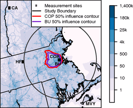
Figure 1. Map of measurement stations in the Boston network including two urban sites: Boston University (BU), 29 m height, and Copley Square (COP), 215 m height; and three boundary sites: Harvard Forest (HF), Canaan, NH (CA), and Martha's Vineyard (MVY). Blue shading represents 2014 average afternoon CO2 emissions. The 90 km-radius circle bounds the region in which emissions were optimized. The red and purple contours encloses 50% of the average 2014 footprint initiated at the COP and BU sites and including only wind directions within plus or minus 40 degrees of the HF or CA boundary sites (Sargent et al., 2018).
Citation
Sargent, M., S.C. Wofsy, and T. Nehrkorn. 2018. CO2 Observations, Modeled Emissions, and NAM-HYSPLIT Footprints, Boston MA, 2013-2014. ORNL DAAC, Oak Ridge, Tennessee, USA. https://doi.org/10.3334/ORNLDAAC/1586
Table of Contents
- Data Set Overview
- Data Characteristics
- Application and Derivation
- Quality Assessment
- Data Acquisition, Materials, and Methods
- Data Access
- References
Data Set Overview
This dataset reports continuous atmospheric measurements of CO2 from two receptor sites and three boundary sites in and around Boston, Massachusetts, USA, that were combined with high-resolution CO2 emissions estimates and the Hybrid Single-Particle Lagrangian Integrated Trajectory (HYSPLIT) model to estimate regional CO2 emissions from September 2013 to December 2014. The HYSPLIT model followed an ensemble of 1,000 particles released at the urban CO2 measurement sites backward in time based on wind fields and turbulence from the North American Mesoscale Forecast System (NAM) at 12-km resolution to the boundary CO2 measurement sites to derive footprint values and CO2 enhancements expected from the prior emissions based on the Anthropogenic Carbon Emissions System (ACES) inventory (Gately and Hutyra, 2018) and the urban-Vegetation Photosynthesis Respiration Model (urbanVPRM) (Hardiman et al., 2017).
This dataset contains three sets of data products: (1) observed hourly mean CO2 observations for two urban receptor sites in Boston, MA (Boston University (BU) and Copley Square (COP)), (2) observed hourly mean CO2 and calculated vertical profiles (50 - 5000 m) for three boundary sites around Boston including Harvard Forest at Petersham, MA (HF), Canaan, NH (CA), and Martha's Vineyard, MA (MVY), and modeled mean boundary CO2 concentrations for particles released from BU and COP, and (3) particle trajectory files including footprint values and CO2 enhancements above boundary CO2 concentrations from the HYSPLIT model.
The observed ΔCO2 was calculated from the difference between urban measurements at BU or COP and estimates of CO2 concentrations in air entering the urban domain, based on boundary values for HF, CA, or MVY and wind direction. The footprint, with units of mixing ratio (ppm) per surface flux (umol m-2 s-1), quantifies the influence of upwind surface fluxes on CO2 concentrations measured at the receptor and is computed by counting the number of particles in a surface-influenced volume and the time spent in that volume. The upstream site assigned to each particle was chosen based on the azimuth at which the particle exited the 90-km radius circle boundary around Boston as it traveled backward in time.
Project: North American Carbon Program (NACP)
The North American Carbon Program (NACP) is a multidisciplinary research program to obtain scientific understanding of North America's carbon sources and sinks and of changes in carbon stocks needed to meet societal concerns and to provide tools for decision makers. Successful execution of the NACP has required an unprecedented level of coordination among observational, experimental, and modeling efforts regarding terrestrial, oceanic, atmospheric, and human components. The project has relied upon a rich and diverse array of existing observational networks, monitoring sites, and experimental field studies in North America and its adjacent oceans. It is supported by a number of different federal agencies through a variety of intramural and extramural funding mechanisms and award instruments.
Related Publication:
Sargent, M., Y. Barrera, T. Nehrkorn, L.R. Hutyra, C.K. Gately, T. Jones, K. McKain, C. Sweeney, J. Hegarty, B. Hardiman, and S.C. Wofsy. 2018. Anthropogenic and biogenic CO2 fluxes in the Boston urban region, PNAS, 115(29), 7491-7496. https://doi.org/10.1073/pnas.1803715115
Related Datasets:
Nehrkorn, T., M. Sargent, S.C. Wofsy, and M. Mountain. 2018. WRF-STILT Particle Trajectories for Boston, MA, USA, 2013-2014. ORNL DAAC, Oak Ridge, Tennessee, USA. https://doi.org/10.3334/ORNLDAAC/1596
Gately, C., and L.R. Hutyra. 2018. CMS: CO2 Emissions from Fossil Fuels Combustion, ACES Inventory for Northeastern USA. ORNL DAAC, Oak Ridge, Tennessee, USA. https://doi.org/10.3334/ORNLDAAC/1501
Acknowledgements:
This research was funded by NASA with grant numbers NNH13CK02C and NNX16AP23G.
Data Characteristics
Spatial Coverage: Massachusetts, Rhode Island, New Hampshire, and area congruent with the ACES emissions inventory, in the Northeastern USA
Spatial Resolution: point
Temporal Coverage: 2013-09-01 to 2014-12-31
Temporal Resolution: Hourly
Study Area (coordinates in decimal degrees). Note that this table provides the coordinates of the overall bounding box for all data files in this dataset and may not correspond exactly to the individual sites.
Table 1. Study areas.
| Site | Westernmost Longitude | Easternmost Longitude | Northernmost Latitude | Southernmost Latitude |
|---|---|---|---|---|
| All sites in the dataset: Boston University (receptor), Copley Square (receptor), Harvard Forest (Petersham, MA), Canaan, NH, and Martha's Vineyard, MA | -72.18 | -70 | 43.709 | 41.35 |
Data File Information
There are 80 files with this dataset, including:
- 32 files in comma-separated (.csv) format, one for each of the 16 months at the BU and COP urban sites with mean hourly observed CO2 concentrations
- 16 files in comma-separated (.csv) format, one for each of the 16 months with observed and calculated CO2 values for the boundary sites
- 32 compressed (*.tar) files, one for each of the 16 months for the BU and COP sites, containing selected hourly particle footprint and CO2 enhancements data in NetCDF (.nc) format. The number of hourly *.nc files ranges from 650-675 for a given month.
Table 2. File names and descriptions.
| File names | Descriptions |
|---|---|
| name_CO2_obs_XXXX_YY.csv | Mean hourly observed CO2 concentrations at the BU and COP sites |
| boundary_CO2_YYYY_MM.csv | Observed CO2 concentrations at HF, CA, and MVY, calculated vertical profiles from 50-5000m for HF, CA, and MVY, and calculated boundary CO2 for BU and COP particle releases |
| hysplit2014x12x42.350Nx71.104Wx00029M-nc.tar | Particle trajectory files including footprint values from the HYSPLIT model run with NAM 12-km meteorology |
Urban Sites Observed CO2 Data
There are 16 files for the Copley Square site and 16 files for the Boston University site; one file for each month from Sept 2013-Dec 2014. The files provide the mean, median and variance of CO2 observations in ppm.
File naming convention:
The files are named name_CO2_obs_YYYY_MM.csv
Where:
name = copley_square or boston_university
YYYY_MM= year and month
Table 3. Variables in the observed CO2 data files: *_CO2_obs_XXXX_YY.csv
| Variable | Units/format | Description |
|---|---|---|
| year | YYYY | Year of observation |
| month | MM | Month of observation |
| day | Day of observation | |
| hour | UTC | Hour of observation in UTC (hr 1= 0:30 - 1:30 data included) |
| mean_CO2 | ppm | Mean observed CO2 concentration |
| median_CO2 | ppm | Median observed CO2 concentration |
| variance_CO2 | ppm | Variance of CO2 observations |
| number_observations | Number of CO2 observations included during hour |
Boundary Sites Observed CO2 Data
There are 16 files, one file for each month from Sept 2013 - Dec 2014, with observed boundary CO2 values for HF, CA and MVY, calculated vertical profiles from 50 - 5000 m for the three boundary sites, and the calculated mean boundary CO2 for particles released from the two urban sites.
File naming convention:
The files are named boundary_CO2_YYYY_MM.csv
Where: YYYY_MM = year and month
Table 4. Variables in the data files boundary_CO2_YYYY_MM.csv.
| Column # | Column header | Units/format | Description |
|---|---|---|---|
| 1 | year | YYYY | Year of observation |
| 2 | month | MM | Month of observation |
| 3 | day | DD | Day of observation |
| 4 | hour | HH (UTC) | Hour of observation, UTC (hr 1= 0:30 - 1:30 data included) |
| 5 | HF_mean_CO2 | ppm | Mean CO2 concentration at Harvard Forest (HF) (ppm) |
| 6 | CA_mean_CO2 | ppm | Mean CO2 concentration at Canaan, NH (CA) (ppm) |
| 7 | MVY_mean_CO2 | ppm | Mean CO2 concentration at Martha's Vineyard, MA (MVY) (ppm) |
| 8 | BU_bound_mean_CO2 | ppm | Modeled mean boundary CO2 concentration (ppm) for all particles released from BU site at this hour. Boundary CO2 for each particle is determined based on angle of exit from region of study (determines boundary site used), time of exit from region of study (determines time at boundary site), and altitude; the contributions of all particles are averaged |
| 9 | COP_bound_mean_CO2 | ppm | Modeled mean boundary CO2 concentration (ppm) for all particles released from COP site at this hour. Boundary CO2 for each particle is determined based on angle of exit from region of study (determines boundary site used), time of exit from region of study (determines time at boundary site), and altitude; the contributions of all particles are averaged |
| 10 | BU_angle_mean | Mean exit angle from 90-km circle around Boston for all particles released from BU site at this hour | |
| 11 | BU_alt_mean | m | Mean altitude of particles (m) at time of exit from 90-km circle around Boston for all particles released from BU site at this hour |
| 12 | BU_time_mean | minutes | Mean time (minutes) particles travel between release and exit from 90-km circle around Boston for all particles released from BU site at this hour. Negative time value indicates minutes before the release time (release time is given by columns 1-4) |
| 13 | COP_angle_mean | Mean exit angle from 90-km circle around Boston for all particles released from COP site at this hour | |
| 14 | COP_alt_mean | m | Mean altitude of particles (m) at time of exit from 90 km circle around Boston for all particles released from COP site at this hour. |
| 15 | COP_time_mean | minute | Mean time (minutes) particles travel between release and exit from 90-km circle around Boston for all particles released from COP site at this hour. Negative time value indicates minutes before the release time (release time is given by columns 1-4) |
| 16-115 | HF_XX | ppm | CO2 concentration (ppm) calculated for our boundary curtain at HF and XX altitude, every 50 m, from 50 to 5000 m. Boundary concentration based on measured HF mean CO2 concentration (column 5) and vertical change based on CO2 flux measurements and Carbon Tracker 2015 gradients as described in Sargent et al. (2018) |
| 116-215 | CA_XX | ppm | CO2 concentration (ppm) calculated for our boundary curtain at CA and XX altitude, every 50 m, from 50 to 5000 m. Boundary concentration based on measured CA concentration (column 6) and vertical change based on Carbon Tracker 2015 gradients as described in Sargent et al. (2018) |
| 216-315 | MVY_XX | ppm | CO2 concentration (ppm) calculated for our boundary curtain at MVY and XX altitude, every 50 m, from 50 to 5000 m. Boundary concentration based on measured MVY concentration (column 7) and vertical change based on Carbon Tracker 2015 gradients as described in Sargent et al. (2018) |
HYSPLIT Particle Trajectories and Footprint Data
These data are footprints, particle trajectories, and CO2 enhancement above boundary concentrations from the HYSPLIT model run with NAM 12-km meteorology. Particle locations are provided as (1) latitude, longitude, and height above ground and (2) latitude and longitude coordinates compatible with the 1-km grid for the ACES emissions inventory.
There are 32 compressed (*.tar) files, one for each of the 16 months for the BU and COP sites, containing selected hourly particle footprint and CO2 enhancements data in NetCDF (.nc) format. The number of hourly *.nc files ranges from 650-675 for a given month.
Tar File Naming Convention:
The files are named by hysplityyyyxmmxlatNxlongWxheightM-nc.tar
Where yyyy = year, mm = month, lat = latitude, long = longitude, height = height A.G.L. of the site, either 29 m (BU) or 155 m (COP).
Example file name: hysplit2014x12x42.350Nx71.104Wx00029M-nc.tar - When uncompressed, this file contains the modeled hourly data for December 2014. The observation was taken at 42.35N, 71.104W at 29 m (BU site) above ground level.
NetCDF file naming convention:
The files follow a similar naming convention, but also include the day and hour of the particle release. However, the *.nc file names begin with "stilt_" rather than "hysplit_" as one might expect. Be assured that the data are from the HYSPLIT model.
The files are named by stiltyyyyxmmxddxhhxlatNxlongWxheightM-nc.tar
Where yyyy = year, mm = month, dd=day of month, hh=hour (UTC), lat = latitude, long = longitude, height = height A.G.L. of the site, either 29 m (BU) or 155 m (COP).
Example file name: stilt2014x12x03x02x42.347Nx71.084Wx00155.nc
This file contains the modeled footprints for December 3, 2014, released at 02 h UTC. The particles were released at 42.347N, 71.084W at 155 m (COP site) above ground level.
Table 5. Variables in the NetCDF data files.
| Variable | Units | Description |
|---|---|---|
| part3d | HYSPLIT particle location array with particle locations saved at 1 minute intervals | |
| part3ddate | days since 2000-01-01 00:00:00 UTC date of part3d | |
| part3dnames | Column names for particle array "part3d"- see Table 6 below | |
| ident | Identifier string |
Table 6. part3d column names.
| part3d.time | Minutes since particle was released; negative value refers to backward trajectory (release time is given by the YYYY, MM, DD, HH of file name) |
| part3d.index | Particle number (1 - 1001) |
| part3d.site | Not used |
| part3d.lat | Latitude of particle's current location |
| part3d.lon | Longitude of particle's current location |
| part3d.agl | Height above ground level (m) of particle's current location |
| part3d.grdht | Elevation of terrain (m) at particle's current location |
| part3d.foot_old | Footprint of particle at current location based on internal HYSPLIT calculation |
| part3d.zi | Planetary boundary layer height (PBLH) at location of particle (m) |
| part3d.dens | Average air density within mixed layer (kg/m3) |
| part3d.lon_m | Longitude on 1 km grid in coordinates compatible with the ACES inventory (Gately and Hutyra, 2018) |
| part3d.lat_m | Latitude on 1-km grid in coordinates compatible with the ACES inventory (Gately and Hutyra, 2018) |
| part3d.foot_mixHt | Footprint of particle at current location based on new mixing height calculation as described in Sargent et al. (2018) |
| part3d.enh_old | CO2 enhancement above boundary concentration associated with this particle at current location, for standard HYSPLIT footprint. Equal to product of foot.old and prior CO2 flux (from ACES (Gately and Hutyra, 2018) 1km anthropogenic inventory and urban VPRM (Hardiman et al.,2017) biogenic inventory) at particle's location and time |
| part3d.enh_mixHt | CO2 enhancement above boundary concentration associated with this particle at current location, part3d. for new mixing height- based footprint. Equal to product of foot.mixHt and prior CO2 flux (from ACES (Gately and Hutyra, 2018) 1km anthropogenic inventory and urban VPRM (Hardiman et al.,2017) biogenic inventory) and at particle's location and time |
| part3d.enh_Xkm | CO2 enhancement above boundary concentration as for enh.mixHt, except prior anthropogenic inventory (ACES) averaged onto X km grid size |
| part3d.enh_bio | CO2 enhancement above boundary concentration as for enh.mixHt, except includes only biogenic fluxes from urbanVPRM (Hardiman et al., 2017) (no anthropogenic fluxes) |
| part3d.enh_uniform | CO2 enhancement above boundary concentration as for enh.mixHt, except prior anthropogenic inventory (ACES) averaged over land in rings bounded at 20, 40, and 90-km around Boston |
Application and Derivation
These data quantify CO2 surface-atmosphere fluxes. Across the globe, it is possible to quantifiably assess the efficacy of greenhouse gas mitigation efforts by developing frameworks similar to the one for this Boston study. For additional details, refer to Sargent et al. (2018).
User Notes:
In reference to the results and analyses presented in the related publication Sargent et al. (2018) -- this dataset must be used in combination with other datasets to produce those results.
For example, to “calculate annual average emissions in the Boston region of 0.92 kg C·m−2·y−1” you would need to use this data set together with the Gately and Hutyra (2018, https://doi.org/10.3334/ORNLDAAC/1501), to calculate anthropogenic emissions. This data set contains everything else needed to reproduce the main reported results in the paper.
To produce some of the secondary results discussed in Sargent et al. (2018) comparing the NAM-HYSPLIT and WRF-STILT models, the https://doi.org/10.3334/ORNLDAAC/1572 and https://doi.org/10.3334/ORNLDAAC/1596 datasets are required.
To calculate “Modeled CO2 “, as the sum of boundary CO2 and modeled ΔCO2, also requires the Gately and Hutyra (2018, https://doi.org/10.3334/ORNLDAAC/1501) dataset. The footprints archived here are multiplied by the prior emissions from Gately to obtain delta CO2 model. Where: (deltaCO2[model] = [sum over all particles] footprint * prior emissions) and (CO2[model] = deltaCO2[model] +CO2[bound]). CO2[bound] is included in the boundary.CO2_YYYY_MM file.
This dataset does provide the factors needed to calculate ΔCO2. Where: (delta CO2[obs] = CO2[obs, BU or COP] - CO2[boundary]). The boundary values are in boundary.CO2_YYYY_MM: "Bound.CO2.BU" and "Bound.CO2.COP", which are boundary values for particles released at either BU or COP and choosing a boundary site based on the wind direction.
Note that using the hysplit files and the altitude level boundary site concentrations "HF_XX", "CA_XX", and "MVY_XX" (in boundary.CO2_YYYY_MM), one could calculate for themselves "Bound.CO2.BU" and "Bound.CO2.COP".
Quality Assessment
Uncertainty in observations was calculated by a bootstrap analysis of daily average concentrations during each season. Boundary CO2 uncertainty was determined from the residuals between our vertically resolved boundary curtain and Carbon Tracker (CT), with the mean difference removed (to remove the effect of any CT bias). Footprint uncertainty was determined by comparison with alternate atmospheric transport and dispersion modeling approaches. For additional details, refer to Sargent et al. (2018).
Data Acquisition, Materials, and Methods
CO2 emissions were quantified in the Boston urban region from September 2013 to December 2014 by modeling the changes in CO2 concentrations as air traveled from the boundary, a 90-km radius around Boston, to the two sites in the urban core, BU and COP.
Observed CO2 Concentrations
Observed CO2 concentrations from the BU and COP sites and from three background sites, HF, CA, and MVY (Figure 1) were used to derive calculated CO2. The atmospheric CO2 concentrations were measured continuously during the period using Picarro cavity ring down spectrometers. The air streams of all instruments were dried using Nafion driers. Hourly averaged concentrations were used for the analysis, with a focus on afternoon hours (11 am to 4 pm local standard time). The urban sites at BU and COP are only 1.7-km apart but sample at 29-m and 215-m above ground level, respectively, providing a direct observation of the surface layer vertical gradient (Sargent et al., 2018).
Table 7. Study site information.
| Site | Longitude | Latitude | Height (meters A.G.L.) |
|---|---|---|---|
| Boston University (BU - receptor) | -71.104 | 42.35 | 29 |
| Copley Square (COP - receptor) | -71.084 | 42.347 | 215 |
| Harvard Forest at Petersham, MA (HF - boundary) | -72.171 | 42.538 | 29 |
| Canaan, NH (CA - boundary) | -72.154 | 43.709 | 100 |
| Martha's Vineyard, MA (MVY - boundary) | -70.527 | 41.35 | 15 |
NAM-HYSPLIT Model Configuration
The modeled CO2 enhancement (ΔCO2) expected from the prior emissions was determined using the HYSPLIT model, which followed an ensemble of 1,000 particles released at the urban measurement sites backward in time based on wind fields and turbulence from NAM at 12-km resolution. HYSPLIT produces an influence function known as the “footprint” (parts per million CO2 per unit flux) that quantifies the particles’ sensitivity to surface emissions, linking upwind surface fluxes to changes in atmospheric concentration at the receptor.
A single multiplicative scaling factor (SF) was calculated for the prior anthropogenic emissions in each season to best match the observed atmospheric gradient.
The HYSPLIT vertical mixing parameter was adjusted from the default of 100 to 50 and the Lagrangian time scale parameter was changed from 100 to 50. These changes increased the footprint by ~15%.
The footprints were convolved with a prior emissions estimate based on the ACES inventory (Gately and Hutyra, 2018) and the urbanVPRM (Hardiman et al., 2017). The convolution of footprints and prior fluxes weights the grid cells in the flux models according to their influence on the measured CO2 enhancement at the urban site.
The observed ΔCO2 was calculated from the difference between urban measurements at BU or COP and estimates of CO2 concentrations in air entering the urban domain, based on measurements at HF, CA, or MVY. The upstream site assigned to each particle was chosen based on the azimuth at which the particle exited the 90-km radius circle around Boston as it traveled backward in time.
Measurements made during times of easterly flow (exit azimuth 0° to 120°) were discarded due to greater uncertainty in modeling sea breezes and lack of a suitable boundary site. The use of all exit angles between sites, except for east winds, were compared with constraints allowing only particles which exited within a certain angle of each site.
Vertical CO2 profiles
To address issues with diurnal variability of CO2 concentrations of air entering the urban domain due to variability of the PBL height and diel variations of upwind fluxes, a method for calculating the CO2 concentration of air entering the urban domain was implemented by constructing a vertical CO2 profile from the observations at each boundary site. At HF, eddy flux measurements made at the same location were used to adjust measured CO2 concentrations at 29 m to their expected value at 200 m (the top of the stratified layer). At CA and MVY, tower measurements were taken as representative of the ground to 200 m.
Above 200 m at all sites, CO2 profiles were constructed using monthly mean vertical gradients from Carbon Tracker CT2015 (CT) (Peters et al., 2007) adjusted to match measurement-based estimates at 200 m. The boundary CO2 concentration for each Lagrangian particle was then determined based on the altitude at which the particle exited the study region, and all particle contributions were averaged.
For additional details, refer to Sargent et al. (2018).
Data Access
These data are available through the Oak Ridge National Laboratory (ORNL) Distributed Active Archive Center (DAAC).
CO2 Observations, Modeled Emissions, and NAM-HYSPLIT Footprints, Boston MA, 2013-2014
Contact for Data Center Access Information:
- E-mail: uso@daac.ornl.gov
- Telephone: +1 (865) 241-3952
References
Gately, C.K., and L.R. Hutyra. 2017. Large uncertainties in urban-scale carbon emissions. J Geophys Res Atmos 122:11242–11260 https://doi.org/10.1002/2017JD027359
Gately, C., and L.R. Hutyra. 2018. CMS: CO2 Emissions from Fossil Fuels Combustion, ACES Inventory for Northeastern USA. ORNL DAAC, Oak Ridge, Tennessee, USA. https://doi.org/10.3334/ORNLDAAC/1501
Hardiman, B.S, J.A. Wang, L.R. Hutyra, C.K. Gately, J.M. Getson, and M.A. Friedl. 2017. Accounting for urban biogenic fluxes in regional carbon budgets. Sci Total Environ 592:366-372. https://doi.org/10.1016/j.scitotenv.2017.03.028
Nehrkorn, T., M. Sargent, S.C. Wofsy, and M. Mountain. 2018. WRF-STILT Gridded Footprints for Boston, MA, USA, 2013-2014. ORNL DAAC, Oak Ridge, Tennessee, USA. https://doi.org/10.3334/ORNLDAAC/1572
Nehrkorn, T., M. Sargent, S.C. Wofsy, and M. Mountain. 2018. WRF-STILT Particle Trajectories for Boston, MA, USA, 2013-2014. ORNL DAAC, Oak Ridge, Tennessee, USA. https://doi.org/10.3334/ORNLDAAC/1596
Peters, W., A.R. Jacobson, C. Sweeney, A.E. Andrews, T.J. Conway, K. Masarie, J.B. Miller, L.M.P. Bruhwiler, G. Petron, A.I. Hirsch, D.E.J. Worthy, G.R. van der Werf, J.T. Randerson, P.O. Wennberg, M.C. Krol, and P.P. Tans. 2007. An atmospheric perspective on North American carbon dioxide exchange: CarbonTracker. Proc Natl Acad Sci USA 104:18925–18930. https://doi.org/10.1073/pnas.0708986104
Sargent, M., Y. Barrera, T. Nehrkorn, L.R. Hutyra, C.K. Gately, T. Jones, K. McKain, C. Sweeney, J. Hegarty, B. Hardiman, and S.C. Wofsy. 2018. Anthropogenic and biogenic CO2 fluxes in the Boston urban region, PNAS, 115(29), 7491-7496. https://doi.org/10.1073/pnas.1803715115