Revision Date: March 11, 2015
Summary:
This data set provides estimates of aboveground biomass (AGB) for defined land cover types within World Wildlife Fund (WWF) ecoregions across the boreal biome of Alaska and western and eastern Canada, roughly between 45 and 70 degrees N. The study focused on within-growing-season data, i.e. leaf-on conditions.
The AGB estimates were derived from a series of models that first related ground-based measured biomass to Portable Airborne Laser System (PALS) LiDAR measurements, and a second set of models that related the airborne estimates of biomass to Geoscience Laser Altimeter System (GLAS) LiDAR canopy structure measurements. The GLAS LiDAR biomass estimates were extrapolated by land cover types and ecoregions across the entire biome area.
The study compiled remotely sensed forest structure data collected in June of 2005 and 2006 from the GLAS LiDAR instrument aboard the NASA Ice, Cloud, and land Elevation (ICESat) satellite and from the PALS airborne instrument flown at various times from 2005-2009 over both the ground plots and the ICESat GLAS flight path. For a consistent biome-level analysis, ecoregions contained within the boreal forest biome were identified by the World Wildlife Fund's (WWF) ecoregion map of the world (Olson et al., 2001). Land cover maps were used to identify land cover types for stratification purposes within eco-regions. Land cover data for Canada were provided by the Earth Observations for Sustainable Development (EOSD) project centered on year 2000, with images from 1999 to 2002. The National Land Cover Data (NLCD) 2001 classification was used for Alaska based on data collected between 1999 and 2004. The ground-based measurements are not provided with this data set.
There are nine data files with this data set which includes the following:
Model Outputs
- The final model output of estimates of AGB for defined land cover types and ecoregions for each of the three regions (Alaska, eastern, and western Canada) in text (.txt) format
- Three GeoTIFF files (.tiff):
- AGB in Mg/ha for all regions combined
- Model-based standard error of AGB in Mg/ha
- Relative error ofAGB in Mg/ha for all three combined regions
Model Inputs
- The input data for the IDL programs that generates the final biomass estimates for each of the three regions (Alaska, eastern, and western Canada) in text (.txt) format
The IDL programs (*.pro) that contains the algorithms to calculate biomass are also provided as companion files, one for each region. In addition, there is a companion file that provides a listing of landcover stratum for Alaska and Canada.
Data Citation:
Cite this data set as follows:
Margolis, H., G. Sun, P.M. Montesano, and R.F. Nelson. 2015. NACP LiDAR-based Biomass Estimates, Boreal Forest Biome, North America, 2005-2006. Data set. Available online [http://daac/ornl.gov/] from Oak Ridge National Laboratory Distributed Active Archive Center, Oak Ridge, Tennessee, USA. http://dx.doi.org/10.3334/ORNLDAAC/1273
Table of Contents:
- 1 Data Set Overview
- 2 Data Characteristics
- 3 Applications and Derivation
- 4 Quality Assessment
- 5 Acquisition Materials and Methods
- 6 Data Access
- 7 References
1. Data Set Overview:
Project: North American Carbon Program (NACP)
The NACP (Denning et al., 2005; Wofsy and Harriss, 2002) is a multidisciplinary research program to obtain scientific understanding of North America's carbon sources and sinks and of changes in carbon stocks needed to meet societal concerns and to provide tools for decision makers. Successful execution of the NACP has required an unprecedented level of coordination among observational, experimental, and modeling efforts regarding terrestrial, oceanic, atmospheric, and human components. The project has relied upon a rich and diverse array of existing observational networks, monitoring sites, and experimental field studies in North America and its adjacent oceans. It is supported by a number of different federal agencies through a variety of intramural and extramural funding mechanisms and award instruments.
AGB was estimated for defined land cover types within WWF ecoregions across the boreal biome of Alaska and western and eastern Canada, roughly between 45 and 70 degrees N. Globally, the boreal forest biome extends in a circumpolar band 13,400 km in length around the Northern Hemisphere roughly between 45 degrees N and 70 degrees N. The study area for this data set is limited to areas of North America (NA). The study focused on within-growing-season data, i.e. leaf-on conditions.
The estimates were derived from a series of models that first related ground-based measured biomass to Portable Airborne Laser System (PALS) LiDAR measurements, and a second set of models that related the airborne estimates of biomass to Geoscience Laser Altimeter System (GLAS) LiDAR canopy structure measurements. The GLAS LiDAR biomass estimates were extrapolated by land cover types and ecoregions across the entire biome area.
The study compiled remotely sensed forest structure data from the GLAS LiDAR instrument aboard the NASA Ice, Cloud, and land Elevation (ICESat) satellite collected in June of 2005 and 2006 and from the PALS airborne instrument flown at various times from 2005-2009 over both the ground plots and the ICESat GLAS flight path. For a consistent biome-level analysis, ecoregions contained within the boreal forest biome were identified by the World Wildlife Fund's (WWF) ecoregion map of the world (Olson et al., 2001). Land cover maps were used to identify land cover types for stratification purposes within eco-regions of the boreal biome in North America. Land cover data for Canada were provided by the Earth Observations for Sustainable Development (EOSD) project centered on year 2000, with images from 1999 to 2002. The National Land Cover Data (NLCD) 2001 classification was used for Alaska based on data collected between 1999 and 2004. Advanced Spaceborne Thermal Emission and Reflection (ASTER) Global Digital Elevation Map (GDEM) Version 1 (V1) data were processed to screen out slopes greater than 20% to reduce the impact of GLAS laser pulse broadening.
2. Data Characteristics:
Spatial Coverage
Boreal forest biome of Alaska and western and eastern Canada, roughly between 45 and 70 degrees N.
Spatial Resolution
1,172 m between sequential GLAS shots which are 60-m in diameter.
Temporal Resolution
One time estimates.
Temporal Coverage
The data cover the period 2005-06-08 to 2006-06-26.
Site boundaries: (All latitude and longitude given in decimal degrees, datum: WGS84)
| Site (Region) | Westernmost Longitude | Easternmost Longitude | Northernmost Latitude | Southernmost Latitude |
|---|---|---|---|---|
| Alaska-Canada (boreal biome of Alaska and western and eastern Canada) | -165 | -53 | 69 | 44 |
Data File Information
There are nine data files with this data set which includes six .txt data files and three GeoTIFF files. The six files include AGB estimates as well as model input variables from GLAS, the ASTER DEM, and land cover maps. The model input variables became one file named Big_Boreal_Burrito or BBB3. The ground-based measurements are not provided with this data set.
The three GeoTIFF (.tiff) files provide: (1) AGB in Mg/ha for all regions combined, (2) model-based standard error of AGB in Mg/ha, and (3) relative error of the AGB in Mg/ha for all three combined regions.
Biomass Data files (.txt format)
AGB data are provided for each individual region--Alaska, eastern Canada, and western Canada. The files contain output data as generated by the IDL programs (*.pro) that contain the algorithms to calculate biomass (the programs are provided as companion files, one for each region).
- The data pertain only to high-graded GLAS shots on slopes <= 20 degrees (avslope).
- Within the model, land cover not classified as wetlands, hardwood, conifer, mixedwood, or burn is equal to zero biomass.
- Total biomass = stems + branches + foliage and is reported in tons/ha.
The data files provide:
(1) AGB for individual ecozones, across flight lines (FL) and systematic samples, for wetlands, hardwood, conifer, mixed wood, and burned areas, as well as estimates from four systematic samples with the number of GLAS shots.
(2) AGB biomass stratum estimates by ecozone.
(3) AGB estimates across all strata (five) and ecozones.
Table 1. Biomass data file names and general descriptions
| FILE NAME | DESCRIPTION |
|---|---|
| alaska_biom20_noshrub.txt | Provides 1, 2, and 3 listed above across 7 ecozones |
| canada_biom20_east_noshrub.txt | Provides 1, 2, and 3 listed above across 6 ecozones |
| canada_biom20_west_noshrub.txt | Provides 1, 2, and 3 listed above across 13 ecozones |
Biomass GeoTIFF Files (.tiff)
Table 2. GeoTIFF file names and general descriptions
| FILE NAME | DESCRIPTION |
|---|---|
| NA_500_ecoLc_rcAGB.tiff | AGB in Mg/ha for all regions combined |
| NA_500_ecoLc_rcRelErr.tiff | Relative error of the AGB in Mg/ha for all three combined regions |
| NA_500_ecoLc_rcSEx2.tiff | Model-based standard error of AGB in Mg/h |
Spatial Data Properties
Spatial Representation Type: Raster
Pixel Depth: 16 bit
Pixel Type: unsigned integer
Compression Type: LZW
Number of Bands: 1
Raster Format: TIFF
Source Type: generic
No Data Value: 255
Scale Factor: 1
Number Columns: 1,4287
Column Resolution: 500 meter
Number Rows: 9,642
Row Resolution: 500 meter
Extent in the items coordinate system
North: 4792125
South: -28875
West: -1251585
East: 5891915
Spatial Reference Properties
Type: Projected
Geographic Coordinate Reference: WGS 84
Projection: WGS_1984_Albers
Open Geospatial Consortium (OGC) Well Known Text (WKT)
PROJCS["WGS_1984_Albers",
GEOGCS["WGS 84",
DATUM["WGS_1984",
SPHEROID["WGS 84",6378137,298.257223563,
AUTHORITY["EPSG","7030"]],
AUTHORITY["EPSG","6326"]],
PRIMEM["Greenwich",0],
UNIT["degree",0.0174532925199433],
AUTHORITY["EPSG","4326"]],
PROJECTION["Albers_Conic_Equal_Area"],
PARAMETER["standard_parallel_1",55],
PARAMETER["standard_parallel_2",65],
PARAMETER["latitude_of_center",50],
PARAMETER["longitude_of_center",-154],
PARAMETER["false_easting",0],
PARAMETER["false_northing",0],
UNIT["metre",1,
AUTHORITY["EPSG","9001"]]]
Model Input Data files (.txt format)
BBB3 in the file names is the abbreviation for the original model input file name used in the IDL program. The files are space delimited and structured for input into the IDL program. There is one companion file for each data file with additional information pertaining to the input data and program codes.
Table 3. Model input data file names and general descriptions
| FILE NAME | DESCRIPTION |
|---|---|
| Alaska_BBB3_hg_L3c_L3f_wPALSbiom.txt | Data file for Alaska in .txt format. For information regarding the program used to derive the estimates, refer to the companion file alaska_glas_5i_noshrub_4Andre.pro |
| Canada_east_BBB3_h3_L3c_L3f_wPALSbiom.txt | Data file for eastern Canada in .txt format. For information regarding the program used to derive the estimates, refer to the companion file can_east_glas_5i_noshrub_4Andre.pro |
| Canada_west_BBB3_h3_L3c_L3f_wPALSbiom.txt | Data file for western Canada in .txt format. For information regarding the program used to derive the estimates, refer to the companion file can_west_glas_5i_noshrub_4Andre.pro |
Model Input Data Variables
Tables 4-7 identify the names, units, and descriptions for all the variables in the model input data files. Each table contains descriptions for the variables and their respective sources.
Table 4. GLAS Variables (GLA01 and GLA14 source). Additional information on GLAS variables can be found at the National Snow & Ice Data Center (NSIDC).
| Variable | Units/format | Description |
|---|---|---|
| rec_ndx | GLAS record index | |
| shotn | Shot number (1 through 40 shots when no pulses are missing) | |
| date | Days since January 1, 2003. | |
| lat | degrees | Latitude in decimal degrees. |
| lngtd | degrees | Longitude in decimal degrees. Negative values for western hemisphere. |
| elev | The elevation of the waveform centroid directly from GLA14. According to the GLAS documentation, this is the “surface elevation with respect to the ellipsoid at the spot location determined by range using the land-specific fitting procedure after all instrument corrections, atmospheric delays and tides have been applied”. | |
| elvdiff | The adjusted “elev” to geoid surface height. | |
| wfl0,lead,trail | m | Waveform height indices. The trailing edge extent (Fig. 1) is most closely related to terrain slope; the leading edge extent (Fig. 1) is related to canopy height variability and must be applied to estimate mean tree height rather than maximum tree height. The trailing edge extent is calculated from the waveform as the height difference between the lowest elevation at which the signal strength of the waveform is half of the maximum signal above the background noise value, and the elevation of the signal end. Similarly, the leading edge extent is determined as the height difference between the elevation of the signal start and the first elevation at which the waveform is half of the maximum signal above the background noise value. Refer to Lefsky et al., 2007 for more detailed explanation |
| MedH | m | Median canopy height |
| MeanH | m | Mean canopy height |
| QMCH | m | Quadratic mean canopy height (Lefsky 1999). If there was difficulty in separating the returns from the canopy and ground, these heights could not be calculated, and were therefore set to zero |
| Centroid, wflen, h14 | m | Waveform centroid (Centroid) and top canopy height (h14) relative to the first Gaussian peak. "wflen" is the distance from signal beginning to ending |
| ht1 | m | The distance from signal beginning to ground peak as calculated from the waveform. |
| ht2 | m | ht1 with a correction for the widening of the ground peak due to slope. |
| ht3 | m | Height that is further corrected for off-nadir looking using beam_ coelev |
| ht4 | m | The height resulting from removing the half width of the laser pulse, so for a bare surface, ht4 should close to zero. |
| fslope | degrees | The angle between vertical and the line from signal beginning to the highest waveform peak. |
| eratio | The ratio of canopy to ground energy. | |
| Senergy | digital counts | The energy from ground. Note that the ratio of canopy energy to total energy is eratio/(1+eratio). |
| h10, h20, h25, h30, h40, h50, h60, h70, h75, h80, h90, h100 | m | Energy indices (relative to ground peak) for each respective percentile. |
| gdpamp | digital counts | Amplitude of the ground peak |
| mjp1loc, mjp2loc, mjp3loc, mjp4loc, mjp5loc, mjp6loc | m | Locations of the six major peaks |
| mjp1amp, mjp2amp, mjp3amp, mjp4amp, mjp5amp, mjp6amp | digital counts | Amplitude of locations of six major peaks |
| satndx | The count of the number of gates in a waveform which have an amplitude greater than or equal to i_satNdxTh (threshold). The value 126 means 126 or more gates are above the saturation index threshold (i_satNdxth). | |
| npk | number | Number of Gaussian peaks retrieved from the waveform. Officially, the number of peaks in the waveform produced by the Gaussian filtering, using alternate parameters. |
| gh1, gh2, gh3, gh4, gh5, gh6 | m | Height of each Gaussian solved for up to six using alternate parameters. The value 99999 signifies missing data if there are not 6 peaks. The algorithm looks for up to six Gaussian peaks in a waveform return but there are often not six peaks to be found. |
| gam1, gam2, gam3, gam4, gam5, gam6 | 0.01 volts | Amplitude of each Gaussian solved for (up to six), using the alternate parameters. Units = 0.01 volts. |
| gs1, gs2, gs3, gs4, gs5, gs6 | 0.001 ns | Width (sigma) of each Gaussian solved for (up to six), using alternate parameters. Units = 0.001 ns. |
| ga1, ga2, ga3, ga4, ga5, ga6 | 0.01 volts x ns | Area under each of the Gaussians solved for (up to six), using alternate parameters. Units = 0.01 volts x ns. |
Table 5. ASTER DEM Variables: The 30-m pixel ASTER DEM was used and divided into the same five regions used for the GLAS data (CD1, CD2, CD3, CD4, AS). The Topographic Modelling function in ENVI was used to compute slopes for a 3 x 3 kernel.The IDL program was developed to locate the slope information for 3 x 3 pixels centered on each quality-filtered GLAS pulse in Acquisitions 2a, 3a, 3c, and 3f.
| Variable | Units/format | Description |
|---|---|---|
| avslope | degrees | Average slope of the nine pixels centered on each GLAS pulse, in degrees. |
| stdslope | degrees | Standard deviation of the slope of the nine pixels centered on each GLAS pulse, degrees. |
| maxslope | degrees | Maximum slope of the nine pixels centered on each GLAS pulse, degrees. |
| minslope | degrees | Minimum slope of the nine pixels centered on each GLAS pulse, degrees. |
Table 6. Land Cover Variables: The EOSD land cover classification for Canada and the NLCD land cover classification for Alaska (see the companion file LandCover_Stratum_Alaska_Canada.txt for classification codes). Resolution is 30 m. The codes for Alaska and Canada can be harmonized as desired. An adapted IDL program was used to locate a 3 x 3 pixel window centered on the GLAS pulse and to calculate the center and dominate LCC for each GLAS pulse. To calculate a viable LCC value, at least 5 of the 9 pixels in the window were required to be vegetated. If there was more than one maximum class in the window and one of the maximum classes was water or otherwise non-vegetated, the vegetated class was selected. In the case of a tie for the dominate vegetated class, the center pixel value was used if it was one of the maximum classes in the 3x3 window. If not, the first value was chosen. The following variables were generated and attached to the GLAS files which eventually became the data input file named BBB3.
| Variable | Units/format | Description |
|---|---|---|
| Can_LCC_Center | The EOSD land cover value for the center of the nine pixels for each GLAS pulse. Set to -9999 when GLAS pulse is located in Alaska. | |
| Can_LCC_Dom | The EOSD dominant land cover class. Set to -9999 when GLAS pulse is located in Alaska. | |
| True_Many_Doms | Flag. Equal to one (1) if there is more than one maximum class, otherwise zero (0). | |
| Max_Class | Number of pixels (1 to 9) in the maximum land cover class. | |
| Conf_pct | percent | Percentage of the nine pixels that were classified as conifer, e.g., 33% |
| Broad_Pct | percent | Percentage of the nine pixels that were classified as broadleaf, e.g., 33%. |
| Mixed_Pct | percent | Percentage of the nine pixels that were classified as mixedwood, e.g., 33%. |
| Shrub_Pct | percent | Percentage of the nine pixels that were classified as shrub, e.g., 33%. |
| Wet_Pct | percent | Percentage of the nine pixels that were classified as wetland, e.g., 33%. |
| AK_LCC_Center | The NLCD land cover value for the center of the nine pixels. Set to -9999 when GLAS pulse is located in Canada. | |
| AK_LCC_Dom | The EOSD dominant land cover class as described above. The percentages were also calculated. Set to -9999 when GLAS pulse is located in Canada. |
Table 7. WWF Ecozone and Other Variables: An IDL program was adapted to extract the WWF ecozone code for each GLAS pulse and attach it to the GLAS data file which eventually became the data input file named BBB3.
| Variable | Units/format | Description |
|---|---|---|
| WWF_EcoID | The WWF ecozone ID | |
| Acquis | The GLAS acquisition number, e.g., 2a = 2.1, 3a = 3.1, 3c=3.3, 3f = 3.6. | |
| Region | Alaska (1.x) or Canada (2.x) | |
| burnyr | Most recent year the area was burned (between and including 2000 - 2006) | |
| burn_jd | Julian day of the burn Note: burn history (year, day) from MODIS burn product - MCD45A1, year 2000 - 2006. | |
| glas_biom_str | metric tons per hectare | Aboveground dry total biomass (including stem, branches, foliage), in metric tons per hectare. |
Companion File Information
Model Programs
The IDL programs (*.pro) that contain the algorithms to calculate biomass from the provided input data are provided as companion files, one for each region. There is also a companion file with the land cover stratum values for Alaska and Canada.
Table 8. Companion Files
| FILE NAME | DESCRIPTION |
|---|---|
| alaska_glas_5i_noshrub_4Andre.pro | Program (.txt format) provides stratified GLAS biomass estimates based on PALS equations across all slopes, slopemax=90 degrees, different ecozones and stratum in Alaska. The model estimates are provided in the data file Alaska_BBB3_hg_L3c_L3f_wPALSbiom.txt |
| can_east_glas_5i_noshrub_4Andre.pro | Program (.txt format) provides stratified GLAS biomass estimates based on PALS equations across all slopes, slopemax=90 degrees, different ecozones and stratum in eastern Canada. The model estimates are provided in the data file Canada_east_BBB3_h3_L3c_L3f_wPALSbiom.txt |
| can_west_glas_5i_noshrub_4Andre.pro | Program (.txt format) provides stratified GLAS biomass estimates based on PALS equations across all slopes, slopemax=90 degrees, different ecozones and stratum in western Canada. The model estimates are provided in the data file Canada_west_BBB3_h3_L3c_L3f_wPALSbiom.txt |
| LandCover_Stratum_Alaska_Canada.txt | NLCD stratum values in Alaska and EOSD stratum values in Canada |
3. Data Application and Derivation:
Our maps establish a baseline for future quantification of circumboreal carbon and the described technique should provide a robust method for future monitoring of the spatial and temporal changes of the aboveground carbon content.
4. Quality Assessment:
A model-based, two-phase estimator developed by Stahl et al. (2011) was used to calculate both sampling variance and model variance. The sampling variance describes the biomass variability among GLAS orbits for a given land cover stratum and model variance describes the uncertainty of the coefficient. Sources of uncertainty, or variance, included sampling variability, model error (i.e., variability of the coefficients), and the covariability among strata across all GLAS orbits (Neigh et al., 2013).
5. Data Acquisition Materials and Methods:
The boreal forest biome extends in a circumpolar band 13,400 km in length around the Northern Hemisphere roughly between 45 degrees N and 70 degrees N. It is bound by tundra to the north and by temperate deciduous forests or savanna/prairie/steppes to the south. Coniferous species of spruce, pine, and fir as well as deciduous larches, birches, alders, and aspens dominate vegetation cover. It contains large quantities of carbon in its vegetation and soils, and research suggests that it will be subject to increasingly severe climate-driven disturbance (Neigh et al., 2013). The study area for this data set included boreal forests in Alaska, western Canada, and eastern Canada.
This study included forest structure data obtained from the the Geoscience Laser Altimeter System (GLAS) LiDAR instrument aboard the NASA Ice, Cloud, and land Elevation (ICESat) satellite, ground-based, and airborne measurements from PALS. The study focused on within-growing-season data, and when available, leaf-on conditions.
The data were incorporated into a model to relate the ground-measured AGB to airborne LiDAR height and canopy density metrics, and another set to relate airborne LiDAR estimates of AGB to GLAS metrics.
Ground-based measurements
The Canadian Forest Service (CFS) provided access to relevant plot data holdings and liaised with provincial and territorial forest resource management agencies obtaining access to geo-located ground plots in Canadian boreal ecoregions. Based on the large area and number of jurisdictions involved, numerous individual researchers, provincial foresters, and industrial foresters measured these plots. Field measurements were collected in Northwest Territories (2006–2008), Saskatchewan (2004–2006), Ontario (2006–2007), and Quebec (2001–2004). The CFS has established species-specific, national-level equations (Lambert, Ung, and Raulier, 2005) that were used to convert ground plot measurements to AGB.
In Alaska, 361 geo-located ground plots were measured by the following U.S. organizations: Forest Service- Kenai Peninsula; Department of Defense- military installations near Fairbanks; and the National Park Service- near Denali N.P., Wrangell - St. Elias N.P., and Yukon- Charley Rivers National Preserve from 2005 to 2007. The United States Forest Service (USFS) compiled the plot locations and associated ground measurements.
Field measurements and observations, made in single radius (circular) plots of 10 or 15-m consisted of: 1) tree species and diameter at breast height (DBH), ± 0.1 cm, for all trees ≥ 3.0 cm in the entire plot; and 2) a sampling of tree height measurements from small, medium, and tall trees for each plot to characterize the range of heights. In general, a 10-m radius plot was employed in dense southern stands (between 50 degrees and 60 degrees N) and a 15-m radius plot was employed in sparser stands above 60 degrees N latitude.
User’s Please Note: The ground-based measurement data described here were essential for the final AGB estimates but are not available for distribution at this time.
Airborne data
The Portable Airborne Laser System (PALS; Nelson, Parker, and Hom, 2003) instrument served as an intermediate sampling tool in North America to extend the spatially limited Canadian National Forest Inventory (NFI) and the U.S. Forest Inventory Analysis (FIA) ground measurements to the continental-scale GLAS observations. Eastern Canada data (Quebec) were collected in the summer 2005, central (Ontario) and western Canada (Northwest Territories and Saskatchewan) were collected in the summer of 2009, and Alaska data were collected in the summer of 2008.
ICESaT data
GLAS waveforms for a given acquisition were examined to assure a strong vegetation signature for potential field measurement, not confounded by clouds or slope. GLAS shots were screened for data that suggested a strong vertical signature of vegetation. GLAS GLA-01 (waveform) and GLA-14 (land) data from ICESaT were accessed and processed. For this study, GLAS data periods included L3c and L3f. L3c period =June 8, 2005 - June 13, 2005; L3f period = June 8, 2006- June 26, 2006. The pulse footprint size = 61 x 47 m. The GLAS data were accessed and distributed by the National Aeronautical and Space Administration (NASA) Goddard Space Flight Center (GSFC) (http://reverb.echo.nasa.gov).
GLAS records the brightness of the 1.064 μm, near-infrared return in one-nanosecond increments as the pulse traverses from the top of the target to the ground. Over trees, the sequential returns recorded for a single pulse provide an initial return from the top of the canopy. Through sequential secondary returns in 15-cm vertical bins, they also provide ranging measurements to sub-canopy layers and the ground as the pulse traverses vertically from top to bottom (Ranson et al., 2004a). Each individual waveform can be analyzed to extract a number of measurements related to the biophysical characteristics of the forest canopy (Yong et al., 2004, Sun et al., 2008). Such measurements include total canopy height, height to sub canopy layers, heights associated with different percentages of pulse energy return, height of median energy (HOME), canopy density (if assumptions are made concerning ground/canopy reflectivity ratio), and canopy height variability (Sun et al., 2008, Yong et al., 2004). These structurally related measurements, in turn, can be related to forest biophysical characteristics of interest such as basal area, timber volume, aboveground biomass, and C stocks (Lefsky et al., 2002, Sun et al., 2008).
GLAS pulse interactions with vegetation on topography with a significant slope can result in pulse broadening, which confounds the interpretation of the influence of the vegetation alone on the waveform (Harding and Carabajal, 2005). ASTER GDEM Version 1 (V1) data were processed to reduce the impact of pulse broadening and all poor-quality data were eliminated.
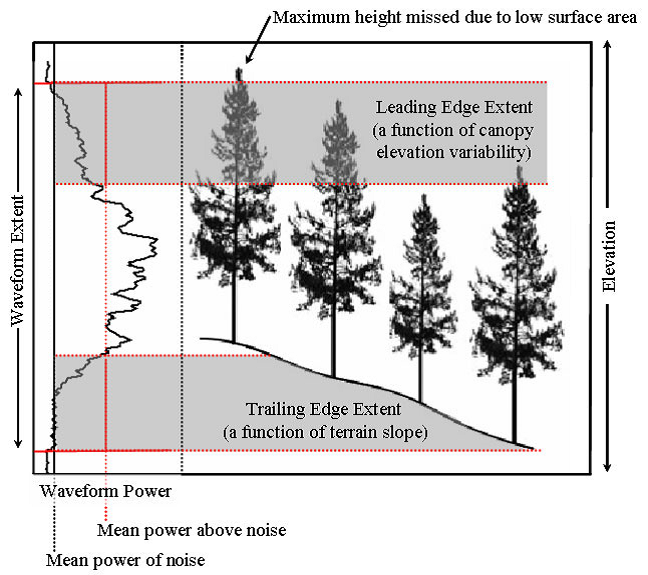
Figure 1. Definition of total waveform, leading and trailing edge extents, and their relationship to forest canopy structure, from Lefsky et al., 2007.
Land cover products for stratification
Land cover maps were used to identify land cover types for stratification purposes within eco-regions of the boreal biome. Land cover data for Canada were provided by the EOSD project, which generated a 25-m land cover map based on Landsat-7 Enhanced Thematic Mapper plus (ETM +) data (centered on year 2000, with images from 1999 to 2002) released in 2006. Trees in this classification were defined as vegetation having a capacity to grow to heights > 5 m.
In Alaska, the 30-m NLCD 2001 classification was used based on Landsat-5 Thematic Mapper (TM) and Landsat-7 ETM + data collected between 1999 and 2004, with a majority of the imagery between 1999 and 2002 (Selkowitz & Stehman, 2011). The NLCD land cover for Alaska is available through the Multi-Resolution Land Characteristics Consortium (MRLC). The MRLC purchased three dates of Landsat imagery for the entire U.S. and similar to EOSD, forests in this classification were defined as having heights > 5 m. Shrubs were excluded for two reasons: 1) the lack of boreal shrub allometric models and plots located in shrub areas; and 2) the lack of sensitivity of GLAS to vegetation < 5-m in height (Nelson, 2010). The two land cover products were updated with recent burned area extents with a combination of fire polygon data obtained from the Canadian Forest Service and Alaska DNR.
For a consistent biome-level analysis, land area was evaluated that was associated with ecoregions contained within the boreal forest biome of North America. The boreal land area, and its component ecoregions, was defined by the World Wildlife Fund's (WWF) ecoregion map of the world (Olson et al., 2001). These ecoregions, along with satellite-based land cover data, were used to create land cover strata, whereby the same land cover falling in different ecoregions was distinguished as unique strata. This stratum designation allowed for further refinement of land cover data and provided a means of grouping ground plots and LiDAR data.
The data were incorporated into models to provide biomass estimations across all strata and included variance estimations. Refer to Neigh et al. (2013) for additional details. The model code for the three individual regions is included with this data set as companion files.
6. Data Access:
These data are available through the Oak Ridge National Laboratory (ORNL) Distributed Active Archive Center (DAAC).
Data Archive Center:
Contact for Data Center Access Information:
E-mail: uso@daac.ornl.gov
Telephone: +1 (865) 241-3952
7. References:
Denning, A.S., et al. 2005. Science implementation strategy for the North American Carbon Program: A Report of the NACP Implementation Strategy Group of the U.S. Carbon Cycle Interagency Working Group. U.S. Carbon Cycle Science Program, Washington, DC. 68 pp.
Harding, D. J., and Carabajal, C. C. (2005). ICESat waveform measurements of within-footprint topographic relief and vegetation vertical structure. Geophysical Research Letters, 32, L21S10.
Lambert, M. C., Ung, C. H., and Raulier, F. (2005). Canadian national tree aboveground biomass equations. Canadian Journal of Forest Research-Revue Canadienne De Recherche Forestiere, 35, 1996–2018.
Lefsky, M.A., M. Keller, Y. Pang, P.B. De Camargo, and M.O. Hunter. (2007). Revised method for forest canopy height estimation from Geoscience Laser Altimeter System waveforms. Journal of Applied Remote Sensing, 1, 013537-013537-013518.
Lefsky, M., Harding, D., Parker, G., Acker, S., and Gower, S. (2002). LiDAR remote sensing of above-ground biomass in three biomes. Global Ecology and Biogeography, 11, 393–399.
Lefsky , M.A., D. Harding, W.B. Cohen and G.G. Parker. 1999. Surface lidar remote sensing of basal area and biomass in deciduous forests of eastern Maryland, USA. Remote Sensing of the Environment. 67:83-98.
Neigh, C.S.R., R.F. Nelson, K.J. Ranson, H.A. Margolis, P. M. Montesano, G. Sun, V. Kharuk, E. Naesset, M.A. Wulder, and H.E. Anderson. 2013. Taking stock of circumboreal forest carbon with ground measurements, airborne and spaceborne LiDAR. Remote Sensing of Environment,137, 276-287 doi:10.1016/j.rse.2013.06.019.
Nelson, R. (2010). Model effects on GLAS-based regional estimates of forest biomass and carbon. International Journal of Remote Sensing, 31, 1359–1372.
Olson, D. M., Dinerstein, E., Wikramanayake, E. D., Burgess, N. D., Powell, G. V. N., Underwood, E. C., et al. (2001). Terrestrial ecoregions of the worlds: A new map of life on Earth. Bioscience, 51, 933–938.
Selkowitz, D. J., and Stehman, S. V. (2011). Thematic accuracy of the National Land Cover Database (NLCD) 2001 land cover for Alaska. Remote Sensing of Environment, 115, 1401–1407.
Stahl, G., Holm, S., Gregoire, T. G., Gobakken, T., Næsset, E., and Nelson, R. (2011). Model-based inference for biomass estimation in a LiDAR sample survey in Hedmark County, Norway. Canadian Journal of Forest Research-Revue Canadienne De Recherche Forestiere, 41, 96–107.
Sun, G., Ranson, K. J., Kimes, D. S., Blair, J. B., and Kovacs, K. (2008). Forest vertical structure from GLAS: An evaluation using LVIS and SRTM data. Remote Sensing of Environment, 112, 107–117.
Yong, P., Sun, G. Q., and Li, Z. Y. (2004). Effects of forest spatial structure on large footprint LiDAR waveform. IGARSS 2004: IEEE International Geoscience and Remote Sensing Symposium Proceedings, Vols. 1–7. (pp. 4738–4741).
Wofsy, S.C., and R.C. Harriss. 2002. The North American Carbon Program (NACP). Report of the NACP Committee of the U.S. Interagency Carbon Cycle Science Program. U.S. Global Change Research Program, Washington, DC. 56 pp.