Documentation Revision Date: 2022-08-30
Dataset Version: 2
Summary
ACES is the first national bottom-up inventory to report hourly fossil fuel carbon dioxide emission (FFCO2) fluxes at a 1-km x 1-km gridded resolution for all major carbon-emitting sectors, using an extensive database of high-resolution spatial proxies.
There are 792 data files with this dataset in NetCDF version 4 (.nc4) format; one file for each month of each year, for the years 2012-2017, for each emissions sector.
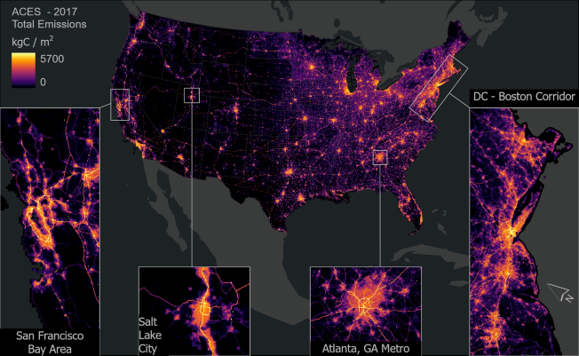
Figure 1. Total emissions for CONUS in the year 2017. Insets show the high-resolution detail of 1 km2 estimates at urban and regional scales. In most metropolitan areas the spatial pattern of emissions is strongly influenced by the onroad emissions sector (from Gately and Hutyra, 2022).
Citation
Gately, C., and L.R. Hutyra. 2022. Anthropogenic Carbon Emission System, 2012-2017, Version 2. ORNL DAAC, Oak Ridge, Tennessee, USA. https://doi.org/10.3334/ORNLDAAC/1943
Table of Contents
- Dataset Overview
- Data Characteristics
- Application and Derivation
- Quality Assessment
- Data Acquisition, Materials, and Methods
- Data Access
- References
- Dataset Revisions
Dataset Overview
The Anthropogenic Carbon Emissions System (ACES) provides estimates of hourly emissions of carbon dioxide produced by fossil fuel combustion across the coterminous United States (CONUS). ACES reports emissions on a 1-km by 1-km spatial grid for every hour of the years 2012 through 2017. ACES emissions are categorized into 10 source sectors: airports and aircraft, commercial and institutional buildings, electric power plants, industrial buildings and facilities, commercial marine vessels, nonroad vehicles and equipment, oil and gas exploration and production wellheads, onroad vehicles, railyards and locomotives, and residential buildings. ACES provides a comprehensive bottom-up estimate of surface fluxes of fossil fuel-derived CO2 and is designed to be used as a prior emission estimate for atmospheric transport models, as a benchmark or comparison for local or regional greenhouse gas inventories, and as a general decision-support tool for climate policy or related analysis.
Project: North American Carbon Program (NACP)
The NACP (Denning et al., 2005; Wofsy and Harriss, 2002) is a multidisciplinary research program to obtain scientific understanding of North America's carbon sources and sinks and of changes in carbon stocks needed to meet societal concerns and to provide tools for decision makers. Successful execution of the NACP has required an unprecedented level of coordination among observational, experimental, and modeling efforts regarding terrestrial, oceanic, atmospheric, and human components. The project has relied upon a rich and diverse array of existing observational networks, monitoring sites, and experimental field studies in North America and its adjacent oceans. It is supported by a number of different federal agencies through a variety of intramural and extramural funding mechanisms and award instruments.
Related Publications:
Gately, C. K. and L. R. Hutyra. 2022. ACES version 2.0, a 1-km gridded hourly inventory of U.S. anthropogenic carbon dioxide emissions for 2012-2017. Nature Scientific Datasets. (in review)
Gately, C. K. andL. R. Hutyra. 2017. Large uncertainties in urban-scale carbon emissions. Journal of Geophysical Research: Atmospheres 122:11242–11260. https://doi.org/10.1002/2017JD027359
Related Datasets:
Gately, C., and L.R. Hutyra. 2018. CMS: CO2 Emissions from Fossil Fuels Combustion, ACES Inventory for Northeastern USA. ORNL DAAC, Oak Ridge, Tennessee, USA. https://doi.org/10.3334/ORNLDAAC/1501
- Version 1 release of the ACES data product for the Northeastern US for the years 2011, 2013, and 2014
Gately, C.K., L.R. Hutyra, and I.S. Wing. 2015. CMS: DARTE Annual On-road CO2 Emissions on a 1-km Grid, Conterminous USA, 1980-2012. ORNL DAAC, Oak Ridge, Tennessee, USA. http://dx.doi.org/10.3334/ORNLDAAC/1285
Acknowledgements
This research was supported primarily by the National Oceanic and Atmospheric Administration (NOAA), grant number NA17OAR4310085 with additional support from National Aeronautics and Spa, grant numbers NNH13CK02C, NNX16AP23G, and NA17OAR4310085
Data Characteristics
Spatial Coverage: The Continental US
Spatial Resolution: 1-km grid
Temporal Coverage: 2012-01-01 to 2017-12-31
Temporal Resolution: Hourly
Site boundaries: (All latitude and longitude given in decimal degrees)
| Site (Region) | Westernmost Longitude | Easternmost Longitude | Northernmost Latitude | Southernmost Latitude |
|---|---|---|---|---|
| CONUS | -128.2675 | 65.3066 | 48.1090 | 23.0132 |
Data File Information
There are 792 data files in NetCDF version 4 (.nc4) format with this dataset. The data reported are emissions of FFCO2 from airports and aircraft, commercial and institutional buildings, electric power plants, industrial buildings and facilities, commercial marine vessels, nonroad vehicles and equipment, oil and gas exploration and production wellheads, onroad vehicles, railyards and locomotives, and residential buildings.
A companion file ACES_V2_Methods_Equations.pdf is included for user’s convenience, which provides the methods with equations referred to in Section 5 of this document.
Table 1. File names and descriptions. YYYYMM in the file names are for each year, 2012 thru 2017, and month, 01-12. For each emissions sector, there are 12 files for each year. There is a "total" file for each year and month covering all sectors.
The no data value = -9999, map units = meters.
| File Name | Description |
|---|---|
| aces_Total_YYYYMM.nc4 | Total hourly CO2 (kg CO2 km-2 h-1) emissions from all sectors |
| aces_Residential_YYYYMM.nc44 | Hourly CO2 (kg CO2 km-2 h-1) emissions from the residential sector |
| aces_Onroad_YYYYMM.nc4 | Hourly CO2 (kg CO2 km-2 h-1 emissions associated from on-road sources |
| aces_Oilgas_YYYYMM.nc4 | Hourly CO2 (kg CO2 km-2 h-1) emissions from the oil and gas production sector |
| aces_Nonroad_YYYYMM.nc4 | Hourly CO2 (kg CO2 km-2 h-1) emissions from mobile sources that are not operating on the public road network (e.g. construction vehicles, agricultural vehicles, lawn and garden equipment) |
| aces_Marine_YYYYMM.nc4 | Hourly CO2 (kg CO2 km-2 h-1) emissions from commercial marine vessels operating in coastal waterways and port areas |
| aces_Elec_YYYYMM.nc4 | Hourly CO2 (kg CO2 km-2 h-1) emissions from electricity generating facilities |
| aces_Air_YYYYMM.nc4 | Hourly CO2 (kg CO2 km-2 h-1) emissions from aircraft taxiing, take-off and landing operations (near-surface only), and other ground-based airport vehicles and on-site stationary combustion sources |
| aces_Commercial_YYYYMM.nc4 | Hourly CO2 (kg CO2 km-2 h-1) emissions from the commercial sector |
| aces_Industrial_YYYYMM.nc4 | Hourly CO2 (kg CO2 km-2 h-1) emissions from the industrial sector (point and non-point combined) |
| aces_Rail_YYYYMM.nc4 | Hourly CO2 (kg CO2 km-2 h-1 emissions from railyard equipment and locomotive operations |
Table 2. Variables in all NetCDF files.
| Variable | Units/format | Description |
|---|---|---|
| flux_co2 | kg CO2 km-2 h-1 | Hourly surface upward mass flux of CO2 (kg CO2 km-2 h-1) |
| lat | decimal degrees | Latitude (degrees north) |
| lon | decimal degrees | Longitude (degrees east) |
| time | hours since 2012-01-01 00:00:00 | Middle of each hour |
| time_bnds | hours since 2012-01-01 00:00:00 | Start and end time for each time stamp |
| x | m | Projection x coordinate |
| y | m | Projection y coordinate |
Application and Derivation
The ACES methodology is designed for easy updating, making it suitable for emissions monitoring under most city, regional, and state greenhouse gas mitigation initiatives. In particular, ACES is useful for the small and medium-sized cities that lack the resources to regularly perform their own bottom-up emissions inventories.
These data could be useful to climate change studies and policies regarding fossil fuel combustion.
Quality Assessment
A comparison of ACES with three of the most commonly used global fossil fuel carbon dioxide emission (FFCO2) inventories shows that even at broad regional scales the overall uncertainty in emissions estimates is as high as 20%. While the ACES inventory itself has a relatively modest total uncertainty of ~8.6%, the overall disagreement between ACES and the major global inventories implies that this uncertainty may be somewhat larger. Two inventories constructed from the same data sources (i.e. ODIAC and FFDAS) report different regional emissions totals (Δ12%) for our domain, emphasizing how minor differences in included source sectors and the downscaling algorithms can produce significant differences at sub-national scales (Gately and Hutyra, 2017).
Data Acquisition, Materials, and Methods
User note: These methods are also provided in the companion file ACES_V2_Methods_Equations.pdf with equations where indicated below.
The first version of the ACES emissions inventory (Northeastern U.S. only) was developed to provide researchers and policymakers in the Northeast U.S. with the ability to quantify and understand trends in FFCO2 emissions at local and regional scales across multiple years (Gately and Hutyra, 2018). This new version of ACES-CONUS represents a substantial expansion of the ACES database to cover the entire CONUS, spanning the years 2012 - 2017, at a 1-km x 1-km hourly resolution. FFCO2 emissions in ACES are derived from publicly available statistics on energy consumption, vehicle activity, industrial processes, and other emission factors. Emissions estimates are provided for ten different source sectors, each with a unique set of spatial and temporal characteristics. Figure 1 shows the total emissions for the CONUS in the year 2017, with insets zoomed into four example urban areas.
Data Sources
A range of input datasets were used to produce the emissions estimates in ACES. The following subsections describe the data inputs and methods used to produce hourly estimates of CO2 fluxes for each ACES sector for CONUS. These methods build from those described extensively by Gately and Hutyra (2017), expanding the geographic scope and updating data sources.
Emissions of CO2 from the residential, commercial, industrial, non-road mobile, aircraft, marine, and rail sectors are derived from a combination of state-level data on fossil fuel consumption by end-use sector reported in the State Energy Data System (SEDS) published by the Energy Information Administration (EIA) and data from the 2014 U.S. Environmental Protection Agency’s (EPA) National Emissions Inventory (NEI). Emissions from point sources, which include electric power generation, industrial facilities, and aircraft take-off and landing operations, were estimated using a combination of data from the NEI and from the EPA Greenhouse Gas Reporting Program (GHGRP). On-road CO2 emissions were obtained from the Database of Road Transportation Emissions (DARTE).
Aircraft and Airport Sector
Aircraft emissions were estimated for near-surface emissions only, covering aircraft taxiing and take-off and landing operations. All emissions for this sector are treated as point sources located at the airport location reported by the NEI.
Annual estimates of carbon monoxide (CO) emissions at each airport are reported in the NEI. CO emissions for aircraft were converted into gallons of jet fuel consumption using emissions factors from the EPA’s WebFIRE database. Total annual consumption of jet fuel and aviation gasoline for each state was obtained from SEDS (codes 'AVACP', 'JFACP', and 'JNACP') for the years 2012-2017. To maintain consistency with SEDS state totals, the NEI-derived estimates of airport-level fuel consumption for 2014 were scaled for each year such that the sum of fuel consumption at all airports in a state matched the SEDS state totals for that year (equation 1 in the companion file NACP_ACES_V2_Methods_Equations). Fuel consumed was then converted to CO2 emissions using emissions factors from the EIA’s Carbon Dioxide Emissions Coefficients Table.
Annual emissions at each airport were then disaggregated to an hourly time structure using take-off and landing data from the Federal Aviation Administration’s Air Traffic Activity System (ATADS). Each day’s share of total annual flights for a given airport in ATADS was used to distribute annual CO2 to daily CO2. ATADS data also provides hourly take-off and landing activity for an average day in each month. The hourly data were used to allocate daily emissions to an hourly pattern for each day in the relevant month and year. For airports without ATADS data, annual emissions at each airport were downscaled using the hourly time structure from the nearest airport in the ATADS system.
Marine Vessels
Coastal and offshore commercial marine vessel CO emissions from NEI were converted to CO2 using emissions factors from EPA with the following assumptions: 1) all marine vessels that burn residual oil as fuel have the emissions characteristics of ‘Ocean-Going Vessels’ and are all 'Medium-Speed Diesel', 2) marine vessels that burn ‘Diesel Fuel’ in the NEI 'Port Emissions' category are 50% ‘Ocean-Going Vessels’ and 50% ‘Harbor Craft’, and 3) marine vessels that burn diesel fuel in the 'Underway emissions' category are 100% ‘Harbor Craft’. Harbor Craft activity was partitioned (both in port and underway) as 25% Category 2 vessels and 75% Category 1 vessels, following EPA9. For Category 1 Harbor Craft, a CO emission factor of 1.5 g / kWh was used, which is the median value for Tier 0 / Tier 1 / Category 1 vessels. A CO emission factor of 1.1 was used for Category 2 Harbor Craft. It was assumed that there are no Tier 2 craft. The CO2 emission factor for all Harbor Craft is 690 g / kWh, as in Table 3.8 of EPA.
Emissions were then assigned to waterways and port areas using the NEI Port and Shipping Lane shapefiles, and then intersected and aggregated to the ACES 1-km grid. Emissions are given a flat hourly time structure, as no data on seasonal, monthly, or diurnal patterns in activity was available. The emissions based on 2014 NEI are replicated for each year in ACES as there were no interannual trend data available at the time of creation.
Point Sources – Electric power plants and industrial facilities
ACES distinguishes between point source emissions from electricity generating facilities and from other type of industrial facilities. The source data for these emissions is obtained from the NEI and the GHGRP. NEI reports annual CO emissions and GHGRP reports annual CO2 emissions. There is overlap between the two datasets, with GHGRP facilities also contained in the NEI dataset. To identify facilities that are duplicated between GHGRP and NEI we constructed as complete a cross-tabulation as possible for all facilities using facility IDs sourced from the EPA’s Facility Registry Service (FRS), the EIA Form 923 database, and crosswalk tables provided by EPA.
After filtering NEI facilities using the facility ID crosswalk, an additional filtering step was performed according to the following criteria:
- Matching facility name, zip code, and state between NEI and GHGRP
- Matching facility address, zip code, and state between NEI and GHGRP
- Matching latitude and longitude between NEI and GHGRP
GHGRP facilities were classified as electric power plants if the ‘sector’ field was equal to ‘Power Plant’. All other GHGRP facilities were assigned to the ACES ‘Industrial’ sector. NEI electric power plant facilities were identified using the included Source Classification Codes. The remaining non-electric power plant NEI point sources were partitioned out for use in other ACES sector estimates, including ‘Aircraft/Airports’, ‘Industrial’, ‘Marine Vessels’, ‘Nonroad Vehicles and Equipment’ and ‘Rail’.
GHGRP facilities directly report annual CO2 emissions, and the data are available for each year in the ACES time series (2012-2017). NEI facilities report CO emissions, and this study was limited to the 2014 NEI vintage. Thus, the NEI fuel types were recoded to match the SEDS fuel types using a crosswalk table. The 2014 NEI fuel consumption data were extrapolated to the years 2012-2013 and 2015-2017 using SEDS state total fuel consumption from the electric power generation end use sector. For each year, the ratio of that year’s state total fuel consumption to the 2014 state total fuel consumption is used as an adjustment factor to the scale each NEI facilities 2014 fuel consumption (equation 2 in the companion file ACES_V2_Methods_Equations.pdf).
The hourly time structure of point source emissions from electric power stations was derived from fuel consumption data reported by a subset of power stations as part of the EPA Air Markets Program Database (AMPD). The hourly heat input was summed to an annual total for each facility, then each hour’s value was divided by this total to generate hourly shares of activity for the facility. Each point source from NEI or GHGRP that was not included in the AMPD was assigned the hourly temporal structure of the nearest AMPD facility. Point location emissions were then intersected with the ACES 1-km grid and spatially aggregated for each hour of the year.
Non-road Vehicles and Equipment
For emissions from vehicles and other fossil fuel powered equipment that do not operate on the public road network (e.g. construction vehicles, agricultural vehicles, lawn and garden equipment), estimates of county-level CO2 were obtained from the NONROAD module included in the EPA Motor Vehicle Emission Simulator (MOVES – version 2014a).
NONROAD provides time-varying emissions estimates for most non-road sources by month and by weekday / weekend for every county in the U.S. A detailed review and comparison of MOVES NONROAD category coverage with other data sources for non-road vehicle activity indicated that the NONROAD model estimates are missing emissions from non-road construction and industrial facility vehicles. Fortunately, data on state-level gasoline consumption for these vehicles are available from the Highway Statistics Series Table MF-24, published annually by the Federal Highway Administration (FHWA). Therefore, the county-level data from the MOVES NONROAD model was supplemented with state-level data on gasoline consumption by construction and industrial facility vehicles from the MF-24 dataset. Table 1 shows the subsectors covered by the MOVES NONROAD and MF-24 datasets.
The state-level MF-24 data were downscaled to county using each county’s fraction of state total CO emissions by subsector in the NEI. (equation 3 in the companion file ACES_V2_Methods_Equations.pdf). MF-24 fuel estimates were then converted to CO2 using emissions factors from EIA. The MF-24 data is only available for the years 2015-2017 with the appropriate subsector categories, as the methodology changed in 2015, and previous years suffer significant data quality issues. Therefore, for the years 2012-2014 the 2015 estimates were used from MF-24. For 2015-2017, the appropriate years’ data were used. The MOVES NONROAD model is very computationally expensive to run and was therefore ran for every county in CONUS for the year 2017 only and use these emissions estimates for all years in ACES.
NONROAD provides estimates of the average daily emissions for an average weekday and an average weekend day for each month of the year. For each of the years 2012 – 2017, the NONROAD output files were expanded to match the calendar year and the appropriate number of weekdays and weekend days. No sub-daily temporal allocation was performed. MF-24 emissions estimates have a flat temporal allocation across all hours of the year.
Non-road emissions are spatially disaggregated from county level using the spatial surrogates developed for the Community Modeling and Analysis System Spatial Allocator (CMAS). The emissions were further disaggregated from the 4-km SMOKE grid down to the 1-km ACES grid using simple areal interpolation.
Table 3. Subsectors covered in the ACES Non-road Sector. CMAS Spatial Surrogate column provides file names for the subsector-specific spatial proxies used to allocate county-level emissions to the CMAS/SMOKE 4-km grid. Surrogate files are available for download at: https://gaftp.epa.gov/Air/emismod/2014/v1/spatial_surrogates/
| Subsector | Source Data | CMAS Spatial Surrogate |
|---|---|---|
| Agriculture | MOVES NONROAD | USA_310_FILL.txt |
| Airport Support | MOVES NONROAD | USA_711_FILL.txt |
| Commercial | MOVES NONROAD | USA_520_FILL.txt |
| Construction | FHWA MF-24 | USA_861_FILL_NORM.txt |
| Industrial | FHWA MF-24 | USA_520_FILL.txt |
| Lawn/Garden | MOVES NONROAD | USA_303_FILL.txt |
| Logging | MOVES NONROAD | USA_890_FILL.txt |
| Oil Field Support | MOVES NONROAD | USA_680_FILL.txt |
| Pleasure Craft | MOVES NONROAD | USA_810_FILL.txt |
| Recreational | MOVES NONROAD | USA_400_FILL.txt |
| Underground Mining | MOVES NONROAD | USA_860_FILL.txt |
On-road Vehicles
ACES on-road emissions are based on annual road-level CO2 emissions estimates reported by the Database of Road Transportation Emissions (DARTE). On-road vehicle emissions are calculated using roadway-level traffic volumes reported by the Highway Performance Monitoring System (HPMS), a traffic monitoring program overseen by the Federal Highway Administration. For each road segment HPMS reports the center-line length in miles, annual average daily traffic (AADT), functional class, urban/rural context, and county. AADT is a measure of the number of vehicles that traverse the road segment on an average day, adjusted for seasonal and day-of-week variation.
For 2012-2017, HPMS became available in shapefile format from FHWA. However, the VMT totals in the 2012-2017 shapefiles do not match the statewide totals reported by the FHWA in the Highway Statistics Series Table VM-2, which was used as a control total in the first release of DARTE. The data were adjusted by calculating the difference in VMT between the HPMS shapefile totals and the Table VM-2 state totals for each functional class and assigned these residual amounts uniformly across that class of roads in each county, based on that county's share of state total VMT for that functional class. This method is the same as was used in the first release of DARTE to assign VMT from the HPMS local road summary files. For further details, see the Supporting Information in Gately et al. (2015).
The HPMS shapefiles also lack representation of the local road network. To maintain consistency across years and to accurately represent the location of emissions on local roads, the data in the HPMS shapefiles was reallocated onto the 2016 TIGER national road network shapefile. Road-segment VMT were aggregated to county scale for the 12 different roadway functional classes included in HPMS, six for urban roads and six for rural roads. State-level VMT data for local roads were then added to each county based on the county’s share of state total VMT of the next higher functional class (minor collectors).
For each year, county, and functional class, annual VMT from HPMS were partitioned into the five vehicle types used by the Highway Statistics Series Table VM-4: Passenger cars, passenger trucks (SUV, pickups, minivans), buses, single-unit trucks, and combination trucks. A calibrated fuel economy and VMT by vehicle type was used to calculate gallons of motor gasoline and diesel fuel consumption, for each year, county, and road functional class. For each road in the database, the annual time series of fuel consumption was then smoothed using a loess (locally estimated scatterplot smoothing) algorithm to reduce inter-annual noise arising from data gaps and periodic road reclassification. For each state, annual fuel consumption for each road was then scaled such that the sum of all roads’ fuel consumption was equal to the published state totals in FHWA Highway Statistics Series Table MF-21 (equation 4 in the companion file ACES_V2_Methods_Equations.pdf). The motor gasoline and diesel fuel consumption were then converted to CO2 emissions using emission factors from EIA. Emissions were assigned to the 2016 Census TIGER/Line road network according to functional class and county, and then aggregated to the ACES 1 x 1- km spatial grid.
To develop a temporal allocation for on-road emissions hourly traffic count data provided by the FHWA Traffic Volume Trends (TVT) program were used. For the year 2012, the TVT data in California was very sparse, so similar data were substituted from the CalTrans Performance Measurement System (PeMS). The total number of traffic monitoring stations with complete hourly data varied year to year from a low of 3,800 in 2013 to a high of 4,900 in 2016, and provided reasonably complete coverage across the U.S.
Hourly vehicle counts for each traffic monitoring station are summed to an annual total, and then each hour is divided by the annual sum for that station to obtain an hourly allocation factor. ACES emissions in each grid cell were assigned the hourly allocation factors of the nearest TVT or PeMS monitoring station.
Oil and Gas Production
CO2 emissions associated with oil and production at the county level were calculated using the EPA Oil and Gas Emission Estimation tool. The tool partitions emissions into four well-type categories: Oil, Gas, Combined Oil & Gas, and Water. The tool reports annual estimates of CO2 emissions from these wellhead types. To allocate these emissions in space the CMAS spatial surrogates for oil and gas wellhead densities (surrogate code 680) were used. The emissions were further disaggregated from the 4-km SMOKE grid down to the 1-km ACES grid. A uniform time structure was used for emissions from this sector, as no temporal allocation information was available. Figure 3 shows the spatial distribution of oil and gas emissions across the CONUS.
Railyards and Trains
Railway CO emissions were obtained from the 2014 NEI and converted to CO2 using emission factors from EPA. Emissions were summed by county and then spatially distributed onto the NEI-provided Rail Line shapefile layer and the 2014 EPA CMV Rail County Shape Fractions for Rail and Commercial Marine.
Point source railyard emissions were obtained by converting NEI estimates of CO at rail yards to CO2 using emissions factors from EPA and EIA. Both the point feature emissions and the linear feature emissions were aggregated together onto the ACES 1-km grid. Emissions were given a flat hourly time structure, as no data on seasonal, monthly, or diurnal patterns in activity was available.
Residential Buildings
State data on annual consumption of fossil fuels by end-use for the residential sector was obtained from the SEDS1. Fuel consumption was then allocated to U.S. Census Block Groups by combining data from several sources:
- The number of households in each Census Block Group that heat with different fuel sources from the American Community Survey (ACS)
- The share of annual household fuel consumption used on space heating versus other end uses such as cooking or heating water from the Residential Energy Consumption Survey (RECS)
- The total square footage of residential units in a Census Block Group extracted from the FEMA HAZUS tool
- The number of ‘heating-degree hours’ a Block Group experienced in each hour of the year, defined as the difference between the hourly average ambient air temperature in a Block Group and 65°F, exclusive to the hours when the average hourly ambient air temperature is less than 65°F.
- Hourly average ambient air temperatures are obtained for each Block Group using the gridded meteorological analysis products from the NOAA Rapid Refresh forecasting system, available at: https://rapidrefresh.noaa.gov
Fuel consumption was first partitioned into two categories: consumption presumed to be influenced by ambient air temperature (i.e. for space-heating purposes), and consumption presumed not to be influenced by air temperature (i.e. hot water heating, cooking, other activities) using the end use shares provided by RECS.
For fuel consumption not influenced by local air temperatures, a flat time structure was given across the year. For temperature-influenced consumption the hourly heating-degree shares were used to assign an hourly time structure, and as part of the allocation process to assign consumption across different Census Block Groups in the state.
For temperature-dependent fuel consumption (superscripted by space) consumption of each fuel (oil, natural gas, liquid propane gas (LPG), coal, and wood) were allocated to Block Groups (equation 5 in the companion file NACP_ACES_V2_Methods_Equations).
The three allocation factors are: (a) the ratio of the number of households in a block group that use fuel f as their primary source of fuel divided by the state-wide total number of households using that fuel, in that year, (b) the ratio of the total number of heating degree hours in the block group that year divided by the average of the total heating degree hours for all block groups in the state (which accounts for variability in climate conditions across a state in a given year), and (c) the fraction of a state’s residential square footage that is located in a given block group. The product of these three allocation factors multiplied by the total fuel consumed in the state results in an estimate of block group fuel consumption. However, since allocation factor (b) is not bounded between 0 and 1, the sums of these block group level fuel consumptions do not total the state fuel consumption. To maintain consistency with the SEDS state totals, block group level estimates are then re-scaled (equation 6 in the companion file NACP_ACES_V2_Methods_Equations)
Hourly fuel consumption is then calculated using each hour of the year’s fraction of total heating degree hours for the block group (equation 7 in the companion file ACES_V2_Methods_Equations.pdf).
For the remaining fuel consumption that is not influenced by ambient temperatures, we allocate to block groups (equation 8 in the companion file ACES_V2_Methods_Equations.pdf).
For this fuel consumption, only the block group’s fraction of households using the fuel and the block group’s share of total state square footage are used to allocate from state totals to block group estimates, whereafter annual totals are allocated to hours by dividing by the total number of hours in the year.
Block group fuel consumption for each fuel type is then summed between the space-heating and other end uses for each hour of the year and converted to CO2 emissions using emissions factors from EIA6. Hourly emissions at block group level are then intersected and aggregated to the ACES 1-km grid. Figure 4 shows annual total emissions from residential sources in 2017 for the CONUS.
Commercial and Institutional Buildings
Fuel consumption for commercial and institutional buildings is also reported annually for each state in SEDS. Fuel consumption was partitioned between space heating (temperature-dependent) and other end uses (non-temperature-dependent) using data from the Commercial Building Energy Consumption Survey (CBECS) Table E7 from 2012, the most recent year that CBECS data is available.
Next, state total fuel consumption was allocated to Census Block Group geographies using a similar method to that of the residential emissions (equation 9 in the companion file NACES_V2_Methods_Equations.pdf).
Again, since allocation factor (b) is not bounded between 0 and 1, the sums of these block group level fuel consumptions do not total the state fuel consumption. To maintain consistency with the SEDS state totals, block group level estimates are re-scaled (equation 10 in the companion file ACES_V2_Methods_Equations.pdf).
Hourly fuel consumption is then calculated using each hour of the year’s fraction of total heating degree hours for the block group (equation 11 in the companion file ACES_V2_Methods_Equations.pdf).
For the remaining fuel consumption that is not influenced by ambient temperatures, we allocate to block groups (as in Equation 12 in the companion file ACES_V2_Methods_Equations.pdf).
For this fuel consumption, only the block group’s fraction of total state commercial building square footage is used to allocate from state totals to block group estimates, whereafter annual block group totals are then allocated to hours by dividing by the total number of hours in the year. Block group fuel consumption for each fuel type is then summed between the space-heating and other end uses for each hour of the year and converted to CO2 emissions using emissions factors from EIA. Hourly emissions at block group level are then intersected and aggregated to the ACES 1-km grid.
Industrial Facilities
The ACES Industrial sector emissions comprise both point- and non-point industrial facilities. “Non-point” facilities are those with emissions levels too small to be included in the GHGRP or the NEI point source emissions datasets. The NEI provides a separate dataset with estimates of CO emissions for these non-point facilities at the county level. These were converted to fuel consumption using emissions factors from EPA.
Industrial point source emissions were estimated using the NEI point layer dataset on CO emissions. Facilities that were not assigned to the electric power generation sector, or the airport, railyard, or nonroad vehicle sectors were designated as industrial and included in this sector. CO emissions were first converted to fuel consumption using emissions factors from the EPA. Total fuel consumption from both point and nonpoint industrial sources was then compared to SEDS state total fuel consumption for the industrial sector. Fuel consumption was then adjusted so that the sum of point and nonpoint estimates equals the SEDS state totals (equation 13 in the companion file ACES_V2_Methods_Equations.pdf). Fuel consumption was then converted into CO2 emissions using emissions factors from EIA.
Temporal allocation of annual emissions to hourly emissions for the point source industrial facilities was done the same way as for point source electric power facilities, using the hourly allocation factors associated with the nearest facility from the EPA AMPD database. For the nonpoint industrial facilities, a flat hourly time structure was used.
Nonpoint industrial emissions were downscaled from county-scale to the SMOKE 4-km grid using the CMAS Spatial Surrogate 505 (industrial land). These estimates were then further downscaled to the ACES 1-km grid. Point source emissions locations were intersected with the ACES 1-km grid and summed with the downscaled nonpoint industrial emissions.
Table 4. Bibliography for data sources as cited above.
|
Data Source Bibliography |
|---|
|
Data Access
These data are available through the Oak Ridge National Laboratory (ORNL) Distributed Active Archive Center (DAAC).
Anthropogenic Carbon Emission System, 2012-2017, Version 2
Contact for Data Center Access Information:
- E-mail: uso@daac.ornl.gov
- Telephone: +1 (865) 241-3952
References
Gately, C. K., and L. R. Hutyra. 2022. ACES version 2.0, a 1-km gridded hourly inventory of U.S. anthropogenic carbon dioxide emissions for 2012-2017. Nature Scientific Datasets. (in review)
Gately, C. K., and L.R. Hutyra. 2017. Large uncertainties in urban-scale carbon emissions. Journal of Geophysical Research: Atmospheres 122:11242–11260. https://doi.org/10.1002/2017JD027359
Gately, C., and L.R. Hutyra. 2018. CMS: CO2 emissions from fossil fuels combustion, ACES inventory for Northeastern USA. ORNL DAAC, Oak Ridge, Tennessee, USA. https://doi.org/10.3334/ORNLDAAC/1501
Gately, C.K., L.R. Hutyra, and I.S. Wing. 2015. Cities, Traffic, and CO2: A multidecadal assessment of trends, drivers, and scaling relationships. Proceedings of National Academy of Sciences 112:4999–5004. https://doi.org/10.1073/pnas.1421723112
Dataset Revisions
| Version | Release Date | Revision Notes |
| 2.0 | 2022-08-30 | The data were extended to CONUS for the period 2012 thru 2017 |
| 1.0 | 2018-04-16 | Original release with data for the Northeastern US for the years 2011, 2013, and 2014 |