Summary:

MAPSS (Mapped Atmosphere-Plant-Soil System) is a landscape to global vegetation distribution model that was developed to simulate the potential biosphere impacts and biosphere-atmosphere feedbacks from climatic change. Model output from MAPSS has been used extensively in the Intergovernmental Panel on Climate Change's (IPCC) regional and global assessments of climate change impacts on vegetation and in several other projects. MAPSS can be run with either a monthly or annual time step and a grid size of 0.5 degree with the example input files provided

The MAPSS model and companion files are distributed in the single compressed file, mapss.tar.gz, and are described below and in MAPSS_Documentation.pdf companion file.

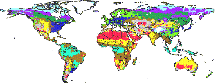
Figure 1. MAPSS Vegetation Distribution (Current Climate)

Conceptual Framework

The conceptual framework for the MAPSS model is that vegetation distributions are, in general, constrained either by the availability of water in relation to transpirational demands, or the availability of energy for growth (Neilson and Wullstein 1983, Neilson et al. 1989, Stephenson 1990, Woodward, 1987). In temperate latitudes, water is the primary constraint while at high latitudes energy is the primary constraint (exceptions occur, of course, particularly in some areas that may be nutrient limited.) The energy constraints on vegetation type and leaf area index (LAI) are currently modeled in MAPSS using a growing degree day algorithm as a surrogate for net radiation (e.g. Botkin et al. 1972, Shugart 1984).

Inputs include the parameters controlling a wide range of ecosystem functions from transpiration factors to vegetation classification, parameters effecting soil functions, monthly total precipitation, mean monthly vapor pressure, mean wind speed, various soil characteristics, and elevation. The input files are described in more detail in the Model Product Description section that follows.

The model calculates the leaf area index of both woody and grass life forms (trees or shrubs, but not both) in competition for both light and water, while maintaining a site water balance consistent with observed runoff (Neilson 1995). Water in the surface soil layer is apportioned to the two life forms in relation to their relative LAIs and stomatal conductance, i.e. canopy conductance, while woody vegetation alone has access to deeper soil water.

Biomes are not explicitly simulated in MAPSS; rather, the model simulates the distribution of vegetation lifeforms (trees, shrubs, grass), the dominant leaf form (broadleaf, needleleaf), leaf phenology (evergreen, deciduous), thermal tolerances and vegetation density (LAI). These characteristics are then combined into a vegetation classification consistent with the biome level (Neilson 1995).

Model Workings

The principal features of the MAPSS model include algorithms for:

1) formation and melt of snow,
2) interception and evaporation of rainfall,
3) infiltration and percolation of rainfall and snowmelt through three soil layers,
4) runoff,
5) transpiration based on LAI and stomatal conductance,
6) biophysical 'rules' for leaf form and phenology,
7) iterative calculation of LAI, and
8) assembly rules for vegetation classification.

Infiltration, and saturated and unsaturated percolation, are represented by an analog of Darcy's Law specifically calibrated to a monthly time step. Water holding capacities at saturation, field potential, and wilting point are calculated from soil texture, as are soil water retention curves (Saxton et al., 1986). Transpiration is driven by potential evapotranspiration (PET) as calculated by an aerodynamic turbulent transfer model based upon Brutsaert's (1982) atmospheric boundary layer (ABL) model (Marks and Dozier, 1992; Marks 1990), with actual transpiration being constrained by soil water, leaf area and stomatal conductance. Stomatal conductance is modulated as a function of PET (a surrogate for vapor pressure deficit) and soil water content (Denmead and Shaw 1962). Canopy conductance (i.e., actual transpiration) is an exponential function of LAI, modulated by stomatal conductance.

Elevated CO2 can affect vegetation responses to climate change through changes in carbon fixation and water-use-efficiency (WUE, carbon atoms fixed per water molecule transpired). The WUE effect is often noted as a reduction in stomatal conductance (Eamus 1991). Since MAPSS simulates carbon indirectly (through LAI), a WUE effect can be imparted directly as a change in stomatal conductance, which results in increased LAI (carbon stocks) and usually a small decrease in transpiration per unit land area.

MAPSS has been implemented at a 10 km resolution over the continental U.S. and at a 0.5 degree resolution globally (Neilson 1995, Neilson 1993a, Neilson and Marks 1994). The model has been partially validated within the U.S. and globally with respect to simulated vegetation distribution, LAI, and runoff (Neilson 1993a; Neilson 1995; Neilson and Marks 1994). MAPSS has also been implemented at the watershed scale (MAPSS-W, 200 m resolution) via a partial hybridization with a distributed catchment hydrology model (Daly 1994, Wigmosta 1994). The model is being archived with ancillary data files for running MAPSS over the conterminous 48 states of the USA at a 0.5-degree latitude by 0.5-degree longitude gridcell resolution.

MAPSS Results

Please see the reference list that follows for papers describing these MAPSS results.

The MAPSS model can simulate the changes in vegetation distribution and runoff under altered climate and carbon dioxide concentration. It simulates both type of vegetation and density, for all upland vegetation from deserts to wet forests.

Overall patterns include a shifting to the north of vegetation, some dieback of boreal forests, particularly along edges of interior grasslands, and a grim outlook for the eastern United States as an area that will likely suffer negative impacts under global warming. There are few "no change" areas within the United States, and the Northwest is an area of uncertainty.

Early stages of global warming could see increases in productivity and density of forests worldwide, as increased carbon dioxide acts as a fertilizer. Continued elevated temperatures, however could strain water resources, in time producing drought-induced stress and broad-scale dieback, with associated wildfire increases.

Increased carbon sequestration from more productive vegetation growth could be offset by pulses of carbon into the atmosphere from increased wildfire.

Integrated assessments of climate change across management sectors ( agriculture, industry, forestry, urban planning, and others) are crucial to preparing for global warming effects. Various alternative futures ought to be considered to maintain management options.

With global warming and the possibility of international greenhouse gas emissions control treaties, the forest management mission could expand further to include carbon sequestration.

Shifting distributions and changing productivity of forests would alter regional forest markets and affect the global forest marketplace. National and regional economies could be altered, with national and global workforce efforts.

Long-term forest management plans are constructed under the assumption of a stable climate. Future expectations within these plans need significant modification to accommodate the range of possibilities under climate change scenarios.

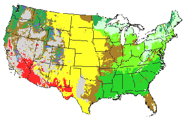
Figure 2. MAPSS Vegetation Distribution (Current Climate)

More information and example outputs can be found at: http://www.fs.fed.us/pnw/corvallis/mdr/mapss/

Data Citation:

Cite this data set as follows:

Neilson, R. P., J. M. Lenihan, D. Bachelet, and R. Drapek. 2007. MAPSS: Mapped Atmosphere-Plant-Soil System Model, Version 1.0. ORNL DAAC, Oak Ridge, Tennessee, USA. http://dx.doi.org/10.3334/ORNLDAAC/853

References:

Botkin, D.B., J.F. Janak, and J.R. Wallis (1972) Rationale, limitation, and assumptions of a northeastern forest growth simulator. IBM Journal of Research and Development 16(2):101-116.

Brutsaert, W. (1982) Evaporation into the Atmosphere, D. Reidel, Dordrecht. Daly, C. (1994) Modeling climate, vegetation, and water balance at landscape to regional scales. Ph.D. Dissertation, Department of General Science, Oregon State University, Corvallis, OR.

Denmead, O.T. and R.H. Shaw (1962) Availability of soil water to plants as affected by soil moisture content and meteorological conditions. Agronomy Journal 54:385-390.

Eamus, D. (1991) The interaction of rising CO2 and temperatures with water use efficiency. Plant, Cell and Environment 14:843-852.

Marks, D. (1990) The sensitivity of potential evapotranspiration to climate change over the continental United States. In: Gucinski, H., Marks, D., & Turner, D.A. (eds.) Biospheric feedbacks to climate change: The sensitivity of regional trace gas emissions, evapotranspiration, and energy balance to vegetation redistribution, pp. IV-1 - IV-31. EPA/600/3-90/078. U.S. Environmental Protection Agency, Corvallis, OR.

Marks, D. & Dozier, J. (1992) Climate and energy exchange at the snow surface in the alpine region of the Sierra Nevada: 2. Snow cover energy balance. Water Resources Research 28: 3043-3054.

Neilson, R.P. (1993a) Vegetation redistribution: A possible biosphere source of CO2 during climatic change. Water, Air and Soil Pollution 70:659-673.

Neilson, R.P. (1995) A model for predicting continental scale vegetation distribution and water balance. Ecol. Appl. 5: 362-385.

Neilson, R.P. and D. Marks (1994) A global perspective of regional vegetation and hydrologic sensitivities from climatic change. Journal of Vegetation Science 5:715-730.

Neilson, R.P., G.A. King, R.L. DeVelice, J. Lenihan, D. Marks, J. Dolph, W.Campbell, and G. Glick (1989) Sensitivity of ecological landscapes to global climatic change. U.S. Environmental Protection Agency, EPA-600-3-89-073, NTIS-PB-90-120-072-AS, Washington, D.C., USA.

Neilson, R.P. and L.H. Wullstein (1983) Biogeography of two southwest American oaks in relation to atmospheric dynamics. Journal of Biogeography 10:275-297.

Saxton, K.E., W.J. Rawls, J.S. Romberger, and R.I. Papendick (1986) Estimating generalized soil-water characteristics from texture. Soil Science Society of America 50:1031-1036.

Shugart, H.H. (1984) A theory of forest dynamics. Springer-Verlag, New York, New York, USA.

Stephenson, N.L. (1990) Climatic control of vegetation distribution: The role of the water balance. The American Naturalist 135:649-670.

Wigmosta, M.S., L.W. Vail, and D.A. Lettenmaier (1994) A distributed hydrology-vegetation model for complex terrain. Water Resources Research 30:1665-1679.

Woodward, F.I. (1987) Climate and plant distribution. Cambridge University Press, London, England.

Model Product Description:

MAPSS Model Distribution

The MAPSS model and companion files are distributed in the single compressed file, mapss.tar.gz

This distribution contains:

1) MAPSS source code files

2) The makefile: Makefile for compiling model code.

3) Example parameter files:  These files hold parameter values controlling a wide range of model functions (site, parameters, and fire_param.dat).

4) Example ancillary data files: Input files of non-climate information for running MAPSS over the conterminous 48 states of the USA at a ½ degree latitude by ½ degree longitude gridcell resolution (elev.nc, soils_scs.nc, and gridpnt.nc).

5) Example climate data files:  Climate data input files (ppt.nc, vpr.nc, tmp.nc, and wnd.nc).

6) Example filter file: The filter file tells MAPSS what model variables to output.

7) Example output files: Examples of monthly and annual output files.

More detailed descriptions of these file types follow.

A note about MAPSS Version 1.0 The MAPSS code has been stable for quite some time. However, for each unique climate data set used as input to the model, the set of parameter files were modified slightly to account for any specific input biases. Publications of these various results would report these minor re-calibrations. Similarly, the basic model produces about 45 unique physiognomic community types that are mapped out. Various projects and publications may have used other classification and aggregation schemes (e.g., 22 classes for VEMAP) to simplify the presentation and discussion, but the basic model code was the same.

Source Code

There are 86 individual code files provided in this distribution. The code consists of two types of files:

• *.c files (29)

• *.h files (57)

Instructions for setting up the MAPSS model, compiling the code, and running the model are given below.

• Command line options and an example command line are given at the end of this section.

• Information about the NetCDF File Format and the Sparse Versus Full Grid Format are also provided.

Input Files

Types of files needed to run MAPSS:

1) Parameter files.

2) Ancillary data files.

3) Climate files.

4) Filter file.

Examples of all these files are included with this distribution.

Parameter Files

There are three parameter files used: "parameters", "site", and "fire_param.dat". These are ASCII text files.

▪ The particular parameter files to be used in any MAPSS run are indicated in the command line with the "-I" parameters.

▪ Following the –I should be a string showing the path to the directory where the "parameters" and "site" files can be found.

▪  The location of the "fire_param.dat" file is hard-coded into the MAPSS code and is set in the file_paths.h file.

Parameters found in all three files are numerical values. Wherever the first column is the start of a numerical value, MAPSS interprets that value as a parameter. Following the parameter value is a parameter name and often some comments. These are there for the benefit of MAPSS program users. MAPSS code ignores them. A "#" is used to indicate comment lines. Blank lines are ignored. For all three parameter files you must have the correct number of parameter entries.

The "parameters" file. The "parameters" file holds parameters controlling a wide range of functions from transpiration calculations to vegetation classification. A "-p" can be used on the command line to indicate the parameters file separately from the site file. Most parameters are explained in Appendix 2 of Neilson (1995).

One parameter that bears special note is the "wue" parameter. Actually there are multiple wue parameters, each for different climate zones and vegetation types. The name wue stands for Water Use Efficiency. The reason these parameters bear special note is they are used in MAPSS for simulating an ecosystem response to enhanced carbon levels. MAPSS does not model photosynthesis and so we cannot directly model a CO2 response as an increase in carbon fixed. But increased CO2 levels are also known to bring about increases in water use efficiency and MAPSS does simulate water use. When running MAPSS for scenarios where CO2 levels were doubled over historical levels, the MAPSS research team set the wue parameters to 0.65. When running over historical CO2 levels, we set the wue parameters to 1.0.

Example records from "parameters" file:

# parameterizations of mapss model # order is critical, do not change order, only values # # # $RCSfile: parameters,v $ # $Revision: 9661 $ # $Date: 2016-12-27 18:36:24 -0500 (Tue, 27 Dec 2016) $ # $Locker: jesse $ 5.0 snow0 temp (C) above which snow fraction equals 0 -7.0 snow1 temp (C) below which snow fraction equals 1 13.0 frost threshold (C) for beginning, end of growing season 10.0 evergreen_productivity_tree Tree productivity for growing season 10.0 evergreen_productivity_shrub used for evergreen/decid decision 10.0 evergreen_productivity_tree_lad 10.0 evergreen_productivity_shrub_lad 600.0 evergreen_gdd growing degree days for mixed (frost based) ...

The "site" file. The site file contains parameters affecting soil functions. A "-s" can be used on the command line to indicate the site file separately from the parameters file.

If you look at the "site" file, you will see that the parameter "WhichSoils" is set to "2", which means scs soils data. When "WhichSoils" is set to "2", MAPSS looks for a soils file called soils_scs.nc. When it is set to "1", MAPSS looks for soils data in the file soils_fao.nc. Alternatively, setting "WhichSoils" to 0 means you don't have to include a soil data input file. MAPSS then will assume that all map-cells are a sandy loam.

 Example records from "site" parameter file:

# # SITES FILE # # site specific inputs to mapss model # Label names are critical, do not change them unless MAPSS is changed internally. # consider soil layer 1 to be upper 500 mm of soil # consider soil layer 2 to be soil at 500 - 1500 mm depth # consider soil layer 3 to be soil below 1500 mm 2 WhichSoils # 0 => NoSoilsData # 1 => FaoSoilsData # 2 => ScsSoilsData 500.0 thickness[SURFACE] 1000.0 thickness[INTERMEDIATE] 1800.0 thickness[DEEP] 0.50 rock_frag_max[SURFACE] 0.50 rock_frag_max[INTERMEDIATE] 0.50 rock_frag_max[DEEP] 0 IgnoreRockFragments # 0 => use rock fragment data # 1 => ignore rock fragment data -0.033 field_potiential ...

The "fire_param.dat" file. This file contains parameters determining the way fire behaves in MAPSS. This file is not subject to change from one run to the next and can in effect be treated as part of the hard MAPSS code. Its location is hard wired for MAPSS in the file_paths.h file (constant FIRE_MODEL_PARMS) and there are no command line parameters for changing this location.

 Example records from "fire_param.dat" parameter file:

3.0 snw0 0.0 snw1 1.0 no_mlt 1.5 melt_b 0.50 k_coeff 0.008 sla_tree_needle 0.014 sla_tree_broad 0.025 sla_shrub 0.019 sla_grass 1000.0 max_lit_accum 1000.0 max_dead_accum 1500.0 sgwood 2500.0 sgherb 2500.0 sg1 109.0 sg10 ...

Ancillary Data Files

The ancillary files hold all the non-climate information needed to describe the region we are simulating. These files are all in NetCDF format and may be either full grid or sparse grid. The names used in this section are what MAPSS is expecting for these files. Examples of each of these were included with this distribution.

The location of the ancillary files is indicated using the "-P" command line parameter. MAPSS is hard coded to look for data in a certain directory. You can see this in the file "file_paths.h" which is included in this distribution. The constant NETCDF_DATA_PATH is used to define this path. Users of this code will need to change this to something more appropriate to their own computer. The name on the command line after the "-P" will be a sub-directory under this base directory.

The example data are for the region bounded by 49N, 25N, 124.5W, and 67W. It is a 48 row by 115 column grid with ½ degree resolution in latitude and longitude. The ancillary files include:

elev.nc- Elevation is measured in meters. These are sparse grid files and are dimensioned as grid x band, where grid is the number of sparse-grid mapcells and band dimensioned as 1. The band dimension is superfluous, but is required by the MAPSS code.

gridpnt.nc- Full grid. Dimensioned as rows x columns. Off-land mapcells are indicated with zeros. On-land mapcells are positive integers sequentially numbered from one. This way every modeled gridcell is given a unique identifying number. This file is used to translate between full and sparse grids.

soils_fao.nc- Soil data.

Sparse grid data dimensioned as grid x band, where there are 10 "bands":

0=mineral_depth (measured in mm),

1=sand[surface](measured  in %),

2=sand[intermediate](%),

3=sand[deep](%),

4=clay[surface](%),  

5=clay[intermediate](%),

6=clay[deep](%),

7=rock_fragment_mineral[surface](%),

8=rock_fragment_mineral[intermediate] (%),

9=rock_fragment_mineral[deep](%).

The three soil depths referred to are:

surface (0-0.5 meters),

intermediate (0.5-1.5 meters), and

deep (greater than 1.5 meters deep).

The name "soils_fao" refers to the fact that for our MAPSS run we stored data from the U.N. Food and Agriculture Organization in this file. If you use this file for your soil data you need to set the "WhichSoils" parameter in the "site" file to "1".

soils_scs.nc- Alternate soil data file.

Same format as soils_fao.nc. We used this format for soil data we picked up from the Soil Conservation Service. If you use this file for your soil data you need to set the "WhichSoils" parameter in the "site" file to "2".

Climate Files

All climate files are sparse grid NetCDF files dimensioned as grid x month. The number of months is always 12 since MAPSS runs on average climate (i.e. average climate for January, average climate for February, etc.).

The climate files include:

ppt.nc- Cumulative monthly precipitation in mm.

tmp.nc- Mean monthly temperature in degrees C.

vpr.nc- Mean monthly vapor pressure in pascals, and

wnd.nc- Mean wind speed in meters/second.

The variables accessed in these files also are called ppt, tmp, wnd, and vpr. MAPSS looks for an attribute for these variables called "scaled". The scaled attribute value is used to modify all data values within the file. So that if the scaled attribute for the temperature file is 100.0, then all values from that file are divided by 100 to yield the actual temperature.

The location of the climate files is indicated using the "-a" command line parameter. The name following the -a is a subdirectory that is located under the ancillary data directory. Since for any region over which we ran the MAPSS model there were often multiple climate scenarios, the data for these scenarios were stored in multiple sub-directories under the ancillary data directory.

NetCDF File Format Basics All climate and ancillary data files are in NetCDF format. For more information on NetCDF look up http://www.unidata.ucar.edu/packages/netcdf. From this website: "NetCDF (network Common Data Form) is an interface for array-oriented data access and a library that provides an implementation of the interface. The NetCDF library also defines a machine-independent format for representing scientific data. Together, the interface, library, and format support the creation, access, and sharing of scientific data." Version 3.6.1 of NetCDF was used. Sparse Versus Full Grid Format As a space saving device, many of the files have been stored in sparse grid format. The full gridded region of any dataset includes many mapcells that are not modeled (example: ocean mapcells). Rather than store many no-value code numbers for all these empty mapcells, a sparse grid file only stores the data for those mapcells that are modelled. Data are stored in the order they appear by row (top to bottom and left to right). An additional file is needed to translate these sparse grid data to full grid when needed. This file has data for all rows and columns. Off-grid mapcells are indicated with zeros and on-grid mapcells are indicated with positive integers. For MAPSS the file "gridpnt.nc" fills this purpose. It is described further in the "Ancillary Files" section.

Output Files

Filter File

The filter file tells MAPSS what model variables to output. The filter file is simply an ASCII text listing of output variables, one per line. An example of a filter file included with this distribution is "out_filter.txt".

• Lines beginning with "#" are ignored by the MAPSS code and can be treated as comment lines.

• Blank lines are also ignored.

• The filter file is indicated in the MAPSS command line call with the "-f" parameter.

• Following the "-f" should be the filter file (full path  included).

The version of MAPSS being distributed here can potentially output 143 variables, but most users would only want a few. Type "mapss -u" once you have MAPSS properly compiled and it will give you a list of all the potential output variables.

 Example records from "out_filter.txt" filter file:

#MAPSS output filter file # #yearly: # class Tree Shrub Grass pet evap at_wood at_grass #monthly output vars: # pet_month evap_month #grass_transpiration_month #woody_transpiration_month

Example Output Files

The output files will be in NetCDF format and will include all of the variables defined in the filter file.

If no “-o” parameter is defined in the command line, then MAPSS defaults to sending annual output to a file called “mapps_out.nc” and to sending monthly output to a file called “mapps_out_monthly.nc”.

Examples of “mapps_out.nc” and “mapps_out_monthly.nc” are included with this distribution.

Steps to Getting MAPSS Operational

To get MAPSS functional you will need to:

 1) Alter NETCDF_DATA_PATH in file_paths.h so that it points to the directory where you intend to store all the climate and ancillary data files.

 2) Also in file_paths.h, alter FIRE_MODEL_PARMS so that it points to the directory where you store the fire parameters file (fire_param.dat).

 3) Make sure all the /local/include/*.h files in the file depend.cc are available.

 4) Create a subdirectory under your NETCDF_DATA_PATH where you will put your ancillary data files. This is the dataset directory. Since these generally describe a geographic region, the directory name generally reflects the region. Example: "usa_48_states".

 5) create one (or more) subdirectories under the dataset directory where you will store the climate data. This is the scenario directory.  These generally are named "historical" or are named for the climate scenario being simulated. Example: "hadcm3_sresa2".

 6) Place your parameter and site file in an appropriate directory (user choice).

 7) Create a filter file and place it in an appropriate directory (user choice).

 8) Modify Makefile so that compiler location, the NetCDF library, etc. are correctly indicated.

 9) Compile and run.

Compiling MAPSS

The version of MAPSS included in this distribution was compiled and run on Sun Microsystems Ultrasparc sun4u machines running on the Solaris 8 operating system. The C compiler was the Sun Workshop Compiler C 5.0. A makefile is provided and MAPSS can be compiled by typing “make all”.

Command Line MAPSS Calls  MAPSS can be run command line. An example command line is given at the end of this document.  Command line options (these can be seen by typing "mapss -h"):   mapss [a:c:C:D:e:f:hI:o:p:P:r:s:Suvz]          filename              If only argument, read command switches from file         -a<scenario>           Alternate data (climate scenario)         -c col1,col2           Begin processing with col1, end with col2         -C<m|p>                Calculate PET (Marks, Penman-Monteith)         -D path                Path to input climate data root directory         -e filename            Error log file name         -f filename            Name of output filter file         -h                      Help         -I path                Directory to search for parameter files         -o filename            Output file name         -p filename            Parameter file name         -r row1,row2           Begin processing with row1, end with row2         -s filename            Site file name         -S                     Set Southern hemisphere <read gridpnt.nc file>         -P dataset             Use netCDF input <dataset> files         -u                     Print output variables available         -v                     Version info and column headings         -z                     Use the grass pet when grass alone

Example Command Line Run

An example run of MAPSS (as done on the MAPSS team computer). See complete set of Command Line Calls below.

 > mapss -Cm -c 0,114 -r 0,47 -I /data/mapss/parameters -P usa_48_states -a historical -f

>      /data/mapss/outputs/out_filter.txt -o /data/mapss/outputs/testrun.nc.

Breakdown:

 "-Cm": This tells MAPSS do use equations derived by Danny Marks to calculate Potential Evapotranspiration. An alternative would be to type     "-Cp", in which case MAPSS would use the equations of Penman-Monteith to make the PET calculation. This would require solar radiation (in 1000.0joule/m2/day) as an additional climate input. Marks PET calculations are suggested for MAPSS.

 "-c 0,114": This tells MAPSS to run over columns 0 to 114.

 "-r 0,47": This tells MAPSS to run over rows 0 to 47.

 "-I /data/mapss/parameters": This tells MAPSS that the site and parameters files will be found in the directory /data/mapss/parameters.

 "-P usa_48_states": This tells MAPSS that the ancillary data will be found in a directory called "usa_48_states", which is directly under the directory identified by the constant NETCDF_DATA_PATH in the MAPSS code. 

 "-a historical": This tells MAPSS that the climate data will be found in a directory called "historical" which will be right under the ancillary data directory.

 "-f /data/mapss/outputs/out_filter.txt": This tells MAPSS that the filter file we will use is called /data/mapss/out_filter.txt (note: the full path is defined for this).

 "-o /data/mapss/outputs/testrun.nc": This tells MAPSS to send output to the file called /data/mapss/outputs/testrun.nc (note: the full path is defined). This output file will be a NetCDF file and will include all of the variables defined in the filter file. If no “-o” parameter is defined in the command line, then MAPSS defaults to sending annual output to a file called “mapps_out.nc” and monthly output to a file called “mapps_out_monthly.nc”

Document Information:

2007/05/24

Document Review Date:

2007/05/24