Documentation Revision Date: 2025-12-03
Dataset Version: 2
Summary
There are 1,584 data files in this dataset, which includes 16 files in cloud-optimized GeoTIFF (COG) format for each Universal Transverse Mercator (UTM) and hemisphere zone. The GeoTIFF files include 11 separate files for the imputed RH metrics—RH10, RH20, RH30, RH40, RH50, RH60, RH70, RH80, RH90, RH95, RH98, as well as five additional files for imputed canopy cover (L2B), AGBD (L4A), sensitivity, GEDI shot number used for imputation (i.e., the single nearest GEDI shot identified using the k-NN or k-nearest neighbors algorithm), and QA indicating pixel quality. In addition, three companion files are provided: a GeoPackage file summarizing imputation performance quality across 10 × 10-km grid cells, a user guide, and the Algorithm Theoretical Basis Document (ATBD).
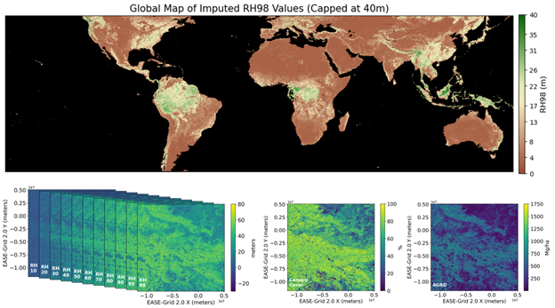
Figure 1. Top figure-Global map showing imputed RH98 metrics. Lower figure-Illustration of imputed waveforms represented by 12 RH metrics (left) with ancillary bands for canopy cover (middle) and aboveground biomass density (right) within a 10-km x 10-km tile.
Citation
Seo, E., S.P. Healey, Z. Yang, R.O. Dubayah, T. De Conto, and J. Armston. 2025. GEDI L4D Imputed Waveforms, Version 2. ORNL DAAC, Oak Ridge, Tennessee, USA. https://doi.org/10.3334/ORNLDAAC/2455
Table of Contents
- Dataset Overview
- Data Characteristics
- Application and Derivation
- Quality Assessment
- Data Acquisition, Materials, and Methods
- Data Access
- References
Dataset Overview
The GEDI Level 4D (L4D) product provides imputed GEDI waveforms for the target year of 2023 at a 30 x 30-m resolution globally between latitudes -51.6 and 51.6 degrees (Figure 1). These waveforms are represented by relative height (RH) metrics at multiple percentile intervals (e.g., RH10, RH20, …, RH95, RH98), similar to those in the GEDI L2A product. GEDI waveform imputation refers to the process of estimating RH values where direct measurements are unavailable. The imputed GEDI waveforms were predicted using the k-nearest neighbors (k-NN) algorithm to choose the single most similar waveform (k = 1) for every pixel based on several variables derived from Landsat time series (CCDC; Zhu et al., 2015) and Global SRTM CHILI (Shuttle Radar Topography Mission Continuous Heat-Insolation Load Index) data (Theobald et al., 2015). Candidate waveforms were acquired 18 April, 2019 to 16 March, 2023. GEDI’s primary measurables represent only a fraction of the ground surface so a product that extends mission measurements over space at high resolution is desirable.
GEDI waveform imputation is performed for each 10 x 10-km grid cell. For every 30-meter pixel, this product contains the imputed GEDI waveform in the form of multiple RH metrics, as well as the corresponding canopy cover and AGBD, derived from the GEDI L2B and L4A products, respectively. This product also provides estimates of the prediction quality for GEDI waveforms, canopy cover, and AGBD within each 10-km grid cell, using root mean square error (RMSE) and the Kolmogorow-Smirnov (KS) test (Fig. 5 and 6). These estimates are based on a randomly selected 20% holdout of high-quality GEDI observations (i.e., validation data). RMSE quantifies the average prediction error for the validation data points, while the KS test evaluates the similarity of distributions of each RH metric in the validation data within the grid cell.
The single nearest neighbor algorithm was chosen for this application to preserve the structure of GEDI’s measurements in two ways. First, at the footprint level, realistic covariance among RH values is maintained by assigning an entire retrieved waveform to each pixel. Second, this approach generally returns predictions with the same distribution as the input reference data. This property is attractive for the mission because GEDI’s waveforms constitute a sample that can be treated as a clustered random sample (Patterson et al., 2019; Dubayah et al., 2022). Other prediction approaches often predict toward the mean of the reference data, which typically minimizes RMSE but which can also underrepresent extreme values.
Project: Global Ecosystem Dynamics Investigation
The Global Ecosystem Dynamics Investigation (GEDI) produces high-resolution laser ranging observations of the 3D structure of the Earth. GEDI’s precise measurements of forest canopy height, canopy vertical structure, and surface elevation greatly advance our ability to characterize important carbon and water cycling processes, biodiversity, and habitat. GEDI was funded as a NASA Earth Ventures Instrument (EVI) mission. It was launched to the International Space Station in December 2018 and completed initial orbit checkout in April 2019.
Related Publications
Dubayah, R.O., J.B. Blair, S. Goetz, L. Fatoyinbo, M. Hansen, S. Healey, M. Hofton, G. Hurtt, J. Kellner, S. Luthcke, J. Armston, H. Tang, L. Duncanson, S. Hancock, P. Jantz, S. Marselis, P.L. Patterson, W. Qi, and C. Silva. 2020. The Global Ecosystem Dynamics Investigation: High-resolution laser ranging of the Earth’s forests and topography. Science of Remote Sensing 1:100002. https://doi.org/10.1016/j.srs.2020.100002
Dubayah, R.O., J. Armston, S.P. Healey, J.M. Bruening, P.L. Patterson, J.R. Kellner, L. Duncanson, S. Saarela, G. Ståhl, Z. Yang, H. Tang, J.B. Blair, L. Fatoyinbo, S. Goetz, S. Hancock, M. Hansen, M. Hofton, G. Hurtt, and S. Luthcke. 2022. GEDI launches a new era of biomass inference from space. Environmental Research Letters 17:095001. https://doi.org/10.1088/1748-9326/ac8694
Duncanson, L., J.R. Kellner, J. Armston, R.O. Dubayah, D.M. Minor, S. Hancock, et al. 2022. Aboveground biomass density models for NASA’s Global Ecosystem Dynamics Investigation (GEDI) lidar mission. Remote Sensing of Environment 270:112845. https://doi.org/10.1016/j.rse.2021.112845
Related Datasets
Dubayah, R.O., M. Hofton, J. Blair, J. Armston, H. Tang, S. Luthcke. 2021. GEDI L2A Elevation and Height Metrics Data Global Footprint Level V002. NASA EOSDIS Land Processes Distributed Active Archive Center, https://doi.org/10.5067/GEDI/GEDI02_A.002
Dubayah, R.O., H. Tang, J. Armston, S. Luthcke, M. Hofton, and J.B. Blair. 2021. GEDI L2B Canopy Cover and Vertical Profile Metrics Data Global Footprint Level V002. NASA Land Processes Distributed Active Archive Center. https://doi.org/10.5067/GEDI/GEDI02_B.002
Dubayah, R.O., J. Armston, J.R. Kellner, L. Duncanson, S.P. Healey, P.L. Patterson, S. Hancock, H. Tang, J. Bruening, M.A. Hofton, J.B. Blair, and S.B. Luthcke. 2022. GEDI L4A Footprint Level Aboveground Biomass Density, Version 2.1. ORNL DAAC, Oak Ridge, Tennessee, USA. https://doi.org/10.3334/ORNLDAAC/2056
Acknowledgments
This work was funded by NASA Earth Ventures Instrument (EVI) mission (contract NNL15AA03C) to the University of Maryland for the development and execution of the GEDI mission (Dubayah, Principal Investigator).
Data Characteristics
Spatial Coverage: Global within a nominal latitude extent of -52 to +52 degrees
Spatial Resolution: 30 m
Temporal Coverage: 2019-04-18 to 2023-03-16
Temporal Resolution: One-time estimate
Study Area: Latitude and longitude are given in decimal degrees
| Site | Westernmost Longitude | Easternmost Longitude | Northernmost Latitude | Southernmost Latitude |
|---|---|---|---|---|
| Global | -180 | 180 | 52.09 | -52.00 |
Data File Information
There are 1,584 data files in this dataset, which includes16 files in cloud-optimized GeoTIFF (*.tif) format for each UTM and hemisphere zone. The GeoTIFF files include 11 separate files for the imputed RH metrics—RH10, RH20, RH30, RH40, RH50, RH60, RH70, RH80, RH90, RH95, RH98, as well as five additional files for imputed canopy cover (L2B), AGBD (L4A), sensitivity, GEDI shot number used for imputation (i.e., the single nearest GEDI shot identified using the k-NN algorithm), and QA indicating pixel quality.
In addition, three companion files are provided: a GeoPackage file summarizing imputation performance quality across 10 × 10-km grid cells, a user guide, and the Algorithm Theoretical Basis Document (ATBD).
GeoTIFF Files
The data files are named GEDI_L4D_UTM<zone>_<hemisphere>_<start date>_<end data>_<variable>.<ext>, where:
- <zone> is the two-digit number of UTM zone ,
- <hemisphere> is the area of terrestrial globe within the corresponding UTM zone ("North" or "South"),
- <start date> is the first date of the GEDI track used for imputation,
- <end date> is the last date of the GEDI track used for imputation,
- <variable> is one of the imputed variables or shot number (e.g., "rh_098", "agbd"; see Table 1),
- <ext> is the file extension ("tif").
Example file name: GEDI_L4D_UTM60_South_20190418_20230316_rh_098.tif
Table 1. Variables and descriptions in corresponding GeoTIFFs.
| Variable Name | Description | Units | Native Data Type | NoData Value |
|---|---|---|---|---|
| rh_xxx | The imputed relative height at the specific pixel, which represents the elevation above ground elevation where <xxx> percentage of the waveform energy has been returned. The valid range of RH values is -21,300 to 21,300. | cm | Signed 16-bit integer (int16) | -32,768 |
| cover_z_000 | The accumulated canopy cover at ground level recorded in the GEDI L2B product from the GEDI shot used for imputation at the corresponding pixel. The values have been scaled to a range of 0 to 100 by multiplying by 100. When a GEDI shot has no corresponding canopy cover value, it is filled with -9999. | percent (%) | Signed 16-bit integer (int16) | -32,768 |
| agbd | The GEDI L4A product's estimate of aboveground biomass density (AGBD) from the GEDI shot used for imputation at the corresponding pixel. When a GEDI shot has no corresponding AGBD value, it is filled with -9999. | Mg ha-1 | Signed 16-bit integer (int16) | -32,768 |
| sensitivity_a2 | The maximum canopy cover, using algorithm 2, that can be penetrated given the signal-to-noise ratio of the waveform (reported as ‘sensitivity’ in the GEDI L2A product) from the GEDI shot used for imputation at the corresponding pixel. See Hofton and Blair (2019). | 1 | Signed 16-bit integer (int16) | -32,768 |
| shot_number | The shot number used for imputation at the corresponding pixel. The 18-digit shot number was parsed from left to right into the following components: orbit (5 digits), beam (2 digits), future (2 digits), granule (1 digit), and shot index (8 digits), resulting in five bands. When the number of digits in the band is less than required, zeros should be padded on the left (e.g., if the values from the five bands are 12466, 6, 0, 3, 619796, the full shot number if 124660600300619796). | 1 | Signed 32-bit integer (int32) | -2147483648 |
| QA | The QA file specifies per-pixel quality information represented by five distinct numeric codes: 0 - No data, as the pixel is outside the zone boundary. 1 - Valid data. 2 - No data due to unavailability of cloud-free CCDC input features. 3 - No data because the nearest shot number was truncated in the Google Earth Engine L2A product. 4 - Pixels corresponding to permanent water bodies within the zone were masked out. |
- | Byte | 0 |
Table 2. Companion files.
| File Name |
Description |
|---|---|
| GEDI_L4D_20190418_20230316_validation_metrics.gpkg | Tile-specific validation information and scores, including RMSE, KS test statistics, and p-values for RH0 to RH100. (see Table 3 for attribute description) |
| GEDI_L4D_Imputed_Waveforms.pdf | This user guide in PDF format. |
| GEDI_L4D_ATBD_V2.pdf | The Algorithm Theoretical Basis Document (ATBD) in PDF format. |
Table 3. Validation metrics file: attributes and descriptions in GEDI_L4D_20190418_20230316_validation_metrics.gpkg.
| Type | Attributes | Description |
|---|---|---|
| Tile information | zone, cellX, cellY, tile_id | Each 10-km tile has information on its UTM zone (‘zone’), row (cellX) and column (cellY) indices relative to the center coordinate (0.0,0.0), and a unique identifier (‘tile_id’). |
| RMSE | rmse_0, rmse_1, ..., rmse_99, rmse_100 |
Root mean square error (RMSE) values for each relative height (RH) metric, from RH0 (rmse_0) to RH100 (rmse_100). |
| rmse_cover, rmse_agbd | RMSE values for canopy cover (rmse_cover) and aboveground biomass density (AGBD) (rmse_agbd). | |
| KS statistic | ks_0, ks_1,..., ks_99, ks_100 |
Kolmogorow-Smirnov (KS) test statistics for each RH metric, from RH0 (ks_0) to RH00 (ks_100). |
| ks_cover, ks_agbd | KS test statistics for canopy cover (ks_cover) and AGBD (ks_agbd). | |
| KS p-value | pval_0, pval _1, ..., pval _99, pval _100 |
KS test p-values for each RH metric, from RH0 (pval_0) to RH00 (pval_100). |
| pval_cover, pval_agbd | KS test p-values for canopy cover (pval_cover) and AGBD (pval_agbd). | |
| Data size | tile_data_size, support_data_size, valid_data_size, valid_data_size_cover, valid_data_size_agbd |
Data size used for building and evaluating k-nearest neighbors (kNN) model. ‘tile_data_size’ is the total number of GEDI shots within the focal tile. ‘support_data_size’ is the total number of GEDI shots within the support tiles defined by the tile-specific tile buffer to ensure at least 2,500 shots. ‘valid_data_size’ is the number of GEDI shots used to validate the kNN model’s performance in predicting RH metrics. ‘valid_data_size_cover’ and ‘valid_data_size_agbd’ are the number of GEDI shots used to validate the kNN model’s predictive performance for canopy cover and AGBD, respectively. |
| Data coverage | contain_valid_data_outside_tile, tile_buffer_size | ‘contain_valid_data_outside_tile’ is a flag indicating whether the validation data comes only from the focal tile (0, False) or also from support tiles (1, True). If the number of GEDI shots in the focal tile is fewer than 500, the validation data is sampled from support tiles. ‘tile_buffer_size’ is the buffer applied at the tile level to define support tiles around the focal tile, ensuring that the total number of qualified GEDI shots is at least 2,500. |
| Mean value from the validation dataset | rh_mean_valid_0, rh_mean_valid_1,…, rh_mean_valid_99, rh_mean_valid_100 |
Mean RH metric values from the validation dataset, which can be used to derive percentage RMSE, from RH0 (rh_mean_valid_0) to RH100 (rh_mean_valid_100) |
| cover_mean_valid, agbd_mean_valid |
Mean canopy cover (cover_mean_valid) and AGBD (agbd_mean_valid) values from the validation dataset, which can be used to derive percentage RMSE. |
Application and Derivation
The GEDI Level 4D (L4D) dataset provides spatially continuous estimates of GEDI waveforms at a 30-meter resolution across the global land surface. These globally imputed GEDI waveforms enable comprehensive forest analysis across scales and can be integrated with local field measurements to support a wide range of applications, including biodiversity assessment and habitat modelling. Representing three-dimensional vegetation profiles, the L4D data offer richer structural information than standard canopy metrics such as height and cover, thereby enhancing the monitoring of forest dynamics, ecosystem structure, and carbon processes worldwide.
The imputed GEDI waveforms are derived from RH metrics in the L2A data, which are processed from observed GEDI waveforms, using a k-NN approach. A raw GEDI waveform is represented by 101 RH metrics—ranging from RH0 to RH100—indicating the elevation above ground corresponding to specific cumulative percentage of the returned laser energy. This sequence of 101 values encodes both the shape of the waveform and key aspects of forest vertical structure. The current version of the L4D product includes RH metrics at 10-percent intervals starting from RH10 (i.e., RH10, RH20, …, Rh95, RH98), along with RH95 and RH98, which are commonly used as proxies for canopy height.
Quality Assessment
A primary goal of GEDI imputation is to preserve the observed distribution of each RH metric within defined local regions, such as 10-km x 10-km spatial tiles. This emphasizes the importance of maintaining the structural integrity of both tall and short trees, ensuring that the imputed data accurately reflect the original variability in vertical forest structure within the specified range. Given that learning-based estimation methods and k-NN with large value of k tend to produce predictions that converge toward average population values—potentially obscuring key characteristics of tall or short trees—the single nearest neighbor was employed. This choice helps better preserve the covariation among related variables, including all RH metrics, canopy cover, aboveground biomass density. Imputing all properties of a single waveform to each pixel also ensures realistic covariance among RH values, an important consideration if different waveform metrics are used together to predict quantities like biomass or fuel model (Fig. 2 and 3).
Evaluation of the imputed waveforms was conducted using a 20% holdout sample from all available high-quality GEDI waveforms. Performance was assessed using KS test and RMSE. The KS test evaluates whether the predicted distribution of each RH metric matches the observed distribution (Fig. 3 and 5), while RMSE quantifies the average error between the predicted and actual RH metric values (Fig. 4 and 6). The companion files provide these evaluation scores for every 10-km x 10-km tile globally between latitudes -51.6 and 51.6 degrees.
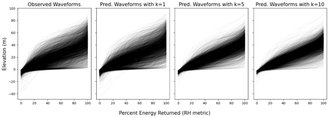
Figure 2. The leftmost figure displays the various forms of recorded waveforms within a 10 x 10-km tile in Olympic National Park, Washington State, USA, while the remaining figures show imputed waveforms generated using different values of k (e.g., the number of nearest neighbors).
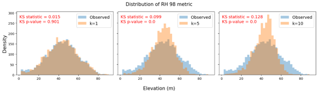
Figure 3. These figures compare the distribution of the RH98 metric derived from the observed waveforms (in blue) with the distribution of predicted RH 98 metric values using different k values (in orange) within the same study area as Figure 2. Minimizing the numbers of neighbors to k=1 results in modeled distributions which much more closely match the real distribution, whereas k-NN with more neighbors compresses the distributions towards the mean value.
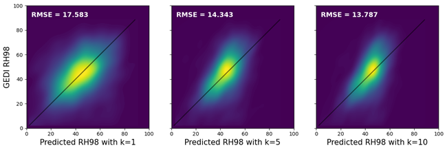
Figure 4. These scatter plots compare observed GEDI RH98 values with predictions from k-NN models (k=1,5,10) presented in Figure 3. The larger the k, the smaller the RMSE, as predictions are compressed toward the mean; however, this not only shrinks the range of the observed values but also leads to overestimation at the lower end (short trees) and underestimation at the upper end (tall trees).
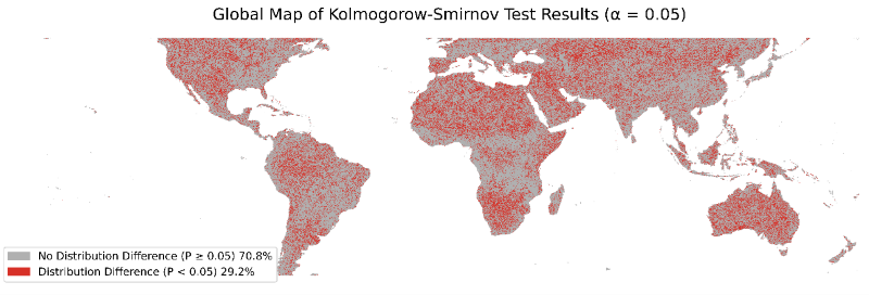
Figure 5. Global map showing the results of the Kolmogorov–Smirnov (KS) test comparing observed and imputed RH98 distributions. Using a significance level of 0.05, 70.8% of tiles show statistically similar distributions, while the remaining 29.2% exhibit significant differences, indicating that the imputed RH98 distribution deviates from the observed distribution in those regions. Both test outcomes are broadly distributed across the globe.
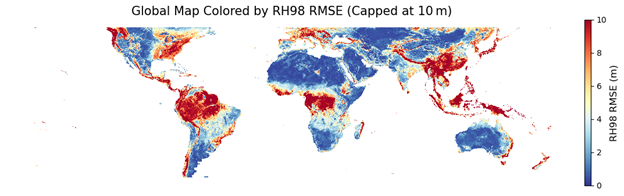
Figure 6. Global map of root mean square error (RMSE) for the RH98 metric, evaluated using the validation dataset.
Data Acquisition, Materials, and Methods
Launched on December 5, 2018, the Global Ecosystem Dynamics Investigation (GEDI) mission provides unprecedented detail on Earth’s forest vertical structure using spaceborne lidar. Mounted on the International Space Station (ISS), GEDI collects globally extensive laser ranging data from orbit, offering comprehensive coverage of Earth’s vegetated landscapes and enabling deeper analysis of ecosystem structure, carbon storage, and biodiversity patterns.
GEDI’s global coverage comprises ground footprints about 25 meters in diameter, measured by eight parallel lidar beams generated by three lasers. These footprints are spaced about 60 meters apart along the orbital path, with approximately 600 meters between adjacent beams in the cross-track direction.
The L4D product is designed to fill the gaps between and across GEDI tracks at 30-meter resolution by leveraging the observed GEDI waveforms.
L2 Footprint Selection
To ensure accurate estimates, the observed GEDI waveforms used as reference must be as free of noise as possible. To achieve this, multiple filtering processes were adopted to use only high-quality GEDI waveforms for the GEDI imputation.
L2A Quality Flags Based Filtering
The initial quality filtering is based on V002 GEDI Level-2A flags. The following criteria are used to filter out low-quality GEDI waveforms:
- ‘quality_flag’ should be equal to 1 (valid surface returns with sensitivity > 0.9)
- ‘degrade_flag’ should be one of 0, 10, 20, 30, 3, 13, 23, 33 (not significantly degraded)
- ‘leaf_off_flag’ should be either 0 (leaf-on) or 255 (unknown)
The degrade flag values were selected by examining geolocation offsets between colocated on-orbit and simulated GEDI waveforms (Hancock et al., 2019).
L4B Sub-orbit Granule Filtering
The second filtering is based on a list of sub-orbit granules excluded as part of quality filtering applied in the GEDI L4B product. This algorithm is detailed in the L4B Algorithm Theoretical Basis Document (ATBD). Any GEDI waveforms belonging to the list of excluded sub-orbit granules were omitted as imputation candidates.
Local Outlier Detection Algorithm
The final filtering step employs a local outlier detection algorithm designed to remove anomalous values that deviate markedly from their surroundings. Unlike L4B’s sub-orbit granule filtering, which excludes entire erroneous sub-orbits, this method identifies individual GEDI waveforms for exclusion. Many of the anomalies eliminated through this process – often due to built structures – would otherwise degrade the spectral relationship used to model tree height. The cost of losing some valid model training data was considered less than the cost of degraded spectral models.
The algorithm is applied to each 10- km x 10-km tile, where it fits a linear regression relating geocoordinates and three environmental variables to the RH98 metric. The fitted linear regression is then used to identify waveforms with unusually abrupt or protruding RH98 metric values relative to their local context. The three environment variables include Near Infrared (NIR) reflectance on the onset of greenness date, NIR on the peak greenness date, and the SRTM-derived Continuous Heat-Insolation Load Index (CHILI) that represent landforms and physiographic patterns. The two greenness dates were derived from the Moderate Resolution Imaging Spectroradiometer (MODIS) data.
10-km x 10-km Tiles
Global 10-km tiles were defined using EASE 2.0 projection starting at the center coordinate (0.0, 0.0). Any tile that does not overlap with any land is excluded from processing, resulting in 1,085,943 tiles globally. Each tile is represented by its row and column index.
k-NN Algorithm
Environmental Covariates
The k-NN algorithm aims to identify for each imputed pixel a location with a high-quality observed GEDI waveform that shares the most similar multivariate characteristics. The L4D product utilizes synthetic Landsat data (Zhu et al., 2015) derived from Continuous Change Detection and Classification (CCDC) . The CCDC algorithms are time series models that fit a mixture of sine and cosine functions to bands of Landsat data (Table 4) to detect land cover change. Using the function fitted to each band, the CCDC algorithms can generate synthetic values for any given date. The synthetic values were used at selected dates as environmental covariates for the k-NN models. Dates were from Moderate Resolution Imaging Spectroradiometer (MODIS) phenology data (Friedl et al., 2022). The MODIS data includes multiple dates representing different stages of land greenness. Two dates were selected – onset of greenup and peak greenness – to characterize sites and derive synthetic band values at these two dates for every 30-meter resolution pixel, as well as for the locations of observed, high-quality GEDI waveforms. The thermal band was excluded. The environmental covariates from CCDC consist of 12 variables: Band 1-5 and 7 for the onset of greenness date (also known as ‘greenup’), and Band 1-5 and 7 for the peak greenness date. Furthermore, the CHILI variable was added to represent terrain and landform characteristics.
Table 4. Primary covariates
| Covariate Name | Description |
|---|---|
| From CCDC at a Greenup Date | |
| Syn_BLUE_Greenup | Synthetic blue band at a greenup date |
| Syn_GREEN_Greenup | Synthetic green band at a greenup date |
| Syn_RED_Greenup | Synthetic red band at a greenup date |
| Syn_NIR_Greenup | Synthetic Near Infrared (NIR) band at a greenup date |
| Syn_SWIR1_Greenup | Synthetic Shortwave Infrared (SWIR1) band at a greenup date |
| Syn_SWIR2_Greenup | Synthetic SWIR2 band at a greenup date |
| From CCDC at a Peak Date | |
| Syn_BLUE_Peak | Synthetic blue band at a peak greenness date |
| Syn_GREEN_Peak | Synthetic green band at a peak greenness date |
| Syn_RED_Peak | Synthetic red band at a peak greenness date |
| Syn_NIR_Peak | Synthetic NIR band at a peak greenness date |
| Syn_SWIR1_Peak | Synthetic SWIR1 band at a peak greenness date |
| Syn_SWIR2_Peak | Synthetic SWIR2 band at a peak greenness date |
| From Global SRTM Continuous Heat-Insolation Load Index | |
| CHILI | SRTM-derived Continuous Heat-Insolation Load Index |
Tile Buffering
The imputation is performed for each 10-km x 10-km tile, with supporting tiles expanded beyond the focal tile by applying at least a one-tile buffer, resulting in a 3 x 3 tile support area centered on the focal tile. The broader support area ensures spatially smooth transitions across tile boundaries. The buffer size can be increased up to 300 x 300 tiles to secure a sufficiently large number of high-quality observed GEDI waveforms. Currently, the criteria is to have at least 2,500 high-quality GEDI waveforms as reference data for the imputation.
Data Access
These data are available through the Oak Ridge National Laboratory (ORNL) Distributed Active Archive Center (DAAC).
GEDI L4D Imputed Waveforms, Version 2
Contact for Data Center Access Information:
- E-mail: uso@daac.ornl.gov
- Telephone: +1 (865) 241-3952
References
Dubayah, R.O., J. Armston, J.R. Kellner, L. Duncanson, S.P. Healey, P.L. Patterson, S. Hancock, H. Tang, J. Bruening, M.A. Hofton, J.B. Blair, and S.B. Luthcke. 2022. GEDI L4A Footprint Level Aboveground Biomass Density, Version 2.1. ORNL DAAC, Oak Ridge, Tennessee, USA. https://doi.org/10.3334/ORNLDAAC/2056
Dubayah, R.O., J. Armston, S.P. Healey, J.M. Bruening, P.L. Patterson, J.R. Kellner, L. Duncanson, S. Saarela, G. Ståhl, Z. Yang, H. Tang, J.B. Blair, L. Fatoyinbo, S. Goetz, S. Hancock, M. Hansen, M. Hofton, G. Hurtt, and S. Luthcke. 2022. GEDI launches a new era of biomass inference from space. Environmental Research Letters 17:095001. https://doi.org/10.1088/1748-9326/ac8694
Dubayah, R.O., M. Hofton, J. Blair, J. Armston, H. Tang, S. Luthcke. 2021. GEDI L2A Elevation and Height Metrics Data Global Footprint Level V002. NASA EOSDIS Land Processes Distributed Active Archive Center, https://doi.org/10.5067/GEDI/GEDI02_A.002
Dubayah, R.O., H. Tang, J. Armston, S. Luthcke, M. Hofton, and J.B. Blair. 2021. GEDI L2B Canopy Cover and Vertical Profile Metrics Data Global Footprint Level V002. NASA Land Processes Distributed Active Archive Center. https://doi.org/10.5067/GEDI/GEDI02_B.002
Dubayah, R., J.B. Blair, S. Goetz, L. Fatoyinbo, M. Hansen, S. Healey, M. Hofton, G. Hurtt, J. Kellner, S. Luthcke, J. Armston, H. Tang, L. Duncanson, S. Hancock, P. Jantz, S. Marselis, P.L. Patterson, W. Qi, and C. Silva. 2020. The Global Ecosystem Dynamics Investigation: High-resolution laser ranging of the Earth’s forests and topography. Science of Remote Sensing 1:100002. https://doi.org/10.1016/j.srs.2020.100002
Duncanson, L., J.R. Kellner, J. Armston, R.O. Dubayah, D.M. Minor, S. Hancock, et al. 2022. Aboveground biomass density models for NASA’s Global Ecosystem Dynamics Investigation (GEDI) lidar mission. Remote Sensing of Environment 270:112845. https://doi.org/10.1016/j.rse.2021.112845
Friedl, M., J. Gray, and D. Sulla-Menashe. 2022. MODIS/Terra+Aqua Land Cover Dynamics Yearly L3 Global 500m SIN Grid V061. NASA Land Processes Distributed Active Archive Center. https://doi.org/10.5067/MODIS/MCD12Q2.061
Hofton, M. and J.B. Blair. 2019. Algorithm Theoretical Basis Document (ATBD) for GEDI Transmit and Receive Waveform Processing for L1 and L2 Products. Version 1.0. Goddard Space Flight Center; Greenbelt, Maryland. https://lpdaac.usgs.gov/documents/581/GEDI_WF_ATBD_v1.0.pdf
Theobald, D. M., D. Harrison-Atlas, W.B. Monahan, and C.M. Albano. 2015. Ecologically-relevant maps of landforms and physiographic diversity for climate adaptation planning. PloS One 10:e0143619. https://doi.org/10.1371/journal.pone.0143619
Zhu, Z., C.E. Woodcock, C. Holden, and Z. Yang. 2015. Generating synthetic Landsat images based on all available Landsat data: Predicting Landsat surface reflectance at any given time. Remote Sensing of Environment 162:67-83. https://doi-org.ornl.idm.oclc.org/10.1016/j.rse.2015.02.009