GEDI-FIA Fusion: Training Lidar Models to Estimate Forest Attributes

This dataset includes interpolated cumulative waveforms, with uncertainties, over national forest inventory (FIA) field plots across the contiguous United States. The predicted waveforms are for the Global Ecosystem Dynamics Investigation (GEDI) instrument, which produces high resolution laser ranging observations of the 3D structure of the Earth. GEDI's data provides precise measurements of forest canopy height, canopy vertical structure, and surface elevation. This dataset also provides R scripts to extract information from user-selected plots and for training linear regression models between GEDI lidar metrics and target forest attributes. The interpolated waveforms are provided in RData and JSON formats. A table of Forest Inventory and Analysis (FIA) plot information is included in comma separated values format

The dataset includes one file in tar.gz format. This tar.gz archive holds three files of R code, one R project file, one file of C++ code, one file in comma separated values format, one text file,and 967 files of interpolated waveforms in both RData and JSON formats.

 

This dataset includes interpolated cumulative waveforms, with uncertainties, over national forest inventory (FIA) field plots (Burrill et al., 2024) across the contiguous United States. The predicted waveforms are for the Global Ecosystem Dynamics Investigation (GEDI) instrument, which produces high resolution laser ranging observations of the 3D structure of the Earth (Dubayah et al., 2020). GEDI’s data provides precise measurements of forest canopy height, canopy vertical structure, and surface elevation. This dataset also provides R scripts to extract information from user-selected plots and for training linear regression models between GEDI lidar metrics and target forest attributes. This dataset was produced using the methods in May et al. (2024).

Project: Global Ecosystem Dynamics Investigation (GEDI)

The Global Ecosystem Dynamics Investigation (GEDI) produces high resolution laser ranging observations of the 3D structure of the Earth. GEDI's precise measurements of forest canopy height, canopy vertical structure, and surface elevation greatly advance our ability to characterize important carbon and water cycling processes, biodiversity, and habitat. GEDI was funded as a NASA Earth Ventures Instrument (EVI) mission. It was launched to the International Space Station in December 2018 and completed initial orbit checkout in April 2019. The lower-level science data products (L1B, L2A, and L2B) are available from the Land Processes DAAC (https://lpdaac.usgs.gov/), and the higher-level products (L3, L4A, and L4B) are available from ORNL DAAC. L3 provides gridded canopy and land surface metrics. L4A and L4B provide aboveground biomass density at footprint and grid levels.

Related Publication: 

May, P.B., R.O. Dubayah, J.M. Bruening, and G.C. Gaines. 2024. Connecting spaceborne lidar with NFI networks: A method for improved estimation of forest structure and biomass. International Journal of Applied Earth Observation and Geoinformation 129:103797. https://doi.org/10.1016/j.jag.2024.103797

Related Dataset:

Dubayah, R., M. Hofton, J. Blair, J. Armston, H. Tang,and S. Luthcke. 2021. GEDI L2A Elevation and Height Metrics Data Global Footprint Level V002. NASA EOSDIS Land Processes Distributed Active Archive Center. https://doi.org/10.5067/GEDI/GEDI02_A.002

Acknowledgements:

This research was supported by NASA’s Global Ecosystem Dynamics Investigation (grant NNL15AA03C) and Carbon Monitoring Systems (grant 80NSSC20K0023) programs.

Spatial Coverage: conterminous United States

Spatial Resolution: ~25 m (the area of a typical GEDI sample footprint)

Temporal Coverage: 2019-03-25 to 2023-03-01

Study Area: Latitude and longitude are given in decimal degrees

Site	Westernmost Longitude	Easternmost Longitude	Northernmost Latitude	Southernmost Latitude
conterminous United States	-132.9538	-57.3678	49.8343	23.2360

Data File Information

The dataset includes one file in tar.gz format: CONUS_GEDI2FIA.tar.gz 
This tar.gz archive holds three files of R code, one R project file, one file of C++ code, one file in comma separated values format, one text file, and 967 files of interpolated waveforms in both RData and JSON formats.

Information about R software and programing language is available at https://www.r-project.org/about.html

The script file washington_biomodel_presentation.R provides a demonstration of these data and the associated scripts. In order to execute as intended, the scripts, FIA_table.csv, and waveform files should be installed in “src”, “data”, and “data/waveform_preds” folders in this structure: 

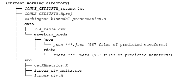
The current working directory must be set while running the R or R Studio software [e.g., setwd()].

The following R library packages are required: dplyr, data.table, matrixcalc, Rcpp, Rcppeigen, BayesLogit, and jsonlite (if using JSON files).

Predicted cumulative waveforms are provided by ecoregion in two alternative formats: RData (a binary file) and JSON. Both formats hold the same data. RData is the default format read by the getRHmetrics.R script; however, that script includes commented lines of code for reading the JSON files. 

Table 1. Files with descriptions. The folder “.” indicates the current working directory.

Folder	File name	Description
. (current working directory)	CONUS_GEDI2FIA.Rproj	An R Project file intended to be opened by R Studio
	CONUS_GEDI2FIA_readme.txt	Basic description of included files.
	washington_biomodel_presentation.R	R script to demonstrate how read the data files and execute the other script files
./data	FIA_table.csv	Text file in comma separated values format that holds FIA plot information (Burrill et al., 2024) for all predicted plots (see Table 2)
./data/waveform_preds/rdata	rdata_***.Rdata	967 files in RData format holding waveform predictions by EPA L4 ecoregion (see Table 3). The [***] gives the EPA L4 code for the associated ecoregion
./data/waveform_preds/json	json_***.json	967 files in JSON format holding waveform predictions by EPA L4 ecoregion (see Table 3). The [***] gives the EPA L4 code for the associated ecoregion
./src	getRHmetrics.R	R script for computing relative height (RH) metrics
	linear_eiv.R	R script that conducts Bayesian linear regression that outputs expect values of regression coefficients with a covariance matrix and expected standard deviations
	linear_eiv_multx.cpp	C++ code supporting calculations in linear_eiv.R script

Table 2. Variables in FIA_table.csv. The first four variables are key fields used to link plot information to other data tables in the larger Forest Inventory and Analysis (FIA) database.

Variable	Units	Description
PLT_CN	-	Unique key field linking plot information to other FIA tables
STATECD	-	State code; Bureau of the Census Federal Information Processing Standards (FIPS) 2-digit code for each State
UNITCD	-	Survey unit code
COUNTYCD	-	County code
PLOT	-	Plot number
INVYR	YYYY	Year of FIA field data collection
puid	-	Unique plot identifier derived by combining the PLOT, UNITCD, COUNTYCD, and STATECD codes: [PLOT_UNITCD_COUNTYCD_STATECD]
US_L4CODE	-	Ecoregion level 4 code from U.S. Environmental Protection Agency
agbd_live_dry_mg_ha	Mg ha-1	Aboveground biomass (dry weight)
LON_PUBLIC	degrees east	Approximate longitude for plot in decimal degrees
LAT_PUBLIC	degrees north	Approximate latitude for plot in decimal degrees

Table 3. Variables in the interpolated waveform files. Only K principal components (PCs) are predicted at the n plots within the ecoregion, where K and n vary by ecoregion file.

Variable	Units	Dimensions	Description
lambda	1	K x 2	The two Box-Cox transformation parameters for each of the K principal components (PC).
mu	m	101	The sample mean of cumulative waveforms within the ecoregion.
PC.bounds	1	2 x K	Minimum and maximum observed values in the ecoregion for each PC used to truncate Monte Carlo samples in getRHmetrics() to avoid numerical instability.
puid	1	n	Unique plot identifier derived by combining the PLOT, UNITCD, COUNTYCD, and STATECD codes: [PLOT_UNITCD_COUNTYCD_STATECD]
rh.eig (values)	m	101	rh.eig provides the eigenvectors and eigenvalues from the sample variance of the 101 RH metrics.
rh.eig (vectors)	m	101 x 101
Zp	1	n x K	The K predicted PCs for each of the n plots.
Zp.var	1	n x K	The K PC prediction variances for each of the n plots.

Monitoring of forest attributes is important for studies of carbon cycling, forest management, and wildlife habitat availability. Light detection and ranging (lidar) is a remote sensing technology for measuring forest structure. NASA’s Global Ecosystem Dynamics Investigation (GEDI) (Dubayah et al., 2020) is an orbital lidar instrument that provides data on forest structure (Dubayah et al., 2021) globally between 54 degrees N and -53 degrees S. However, further analysis is needed to convert GEDI’s waveform data into measurements of forest attributes. The code in this dataset demonstrates how to build regression models for that purpose.

The dataset contains predicted cumulative waveforms along with associated standard errors, and the requisite information to compute other quantification of uncertainty, such as credible intervals. The accuracy of these reported uncertainties was tested in May et al. (2024).

For each ecoregion, a sample mean vector and sample covariance matrix for all quality flagged, observed cumulative waveforms (RH 0-100) was computed. The eigen decomposition of this covariance matrix was computed, yielding the variable rh.eig, which contains the eigenvectors and eigenvalues. The first K eigenvectors containing at least 99.99% of the variance were selected for spatial interpolation. The observed cumulative waveforms were projected onto these K eigenvectors, yielding K principal components (PCs). These PCs were transformed to be approximately normally distributed with a Box-Cox transformation. Each column of variable lambda contains the maximum likelihood estimate for the two Box-Cox parameters (an exponent and translation parameter). The K transformed PCs were interpolated onto the FIA plot locations using a spatial model, yielding a prediction (Zp), and a prediction variance (Zp.var).

A probability distribution for the predicted waveform can be constructed using Monte Carlo methods, as done in the getRHmetrics() function in “./src/getRHmetrics.R'”. The true transformed PCs are assumed to be normally distributed with mean Zp and variance Zp.var. Random samples are drawn from this normal distribution, adding the variance from the not-interpolated 101–K transformed PCs. These samples are back-transformed through the inverse of the Box-Cox transformation, yielding random samples of the original PCs with no transformation. These samples are multiplied by the eigenvector matrix to yield random samples of the cumulative waveform. 

See May et al. (2024) for a more detailed description of the above methods.

The interpolated waveform files in the folder “./data/waveform_preds/'' are waveform predictions by ecoregion. These files can be opened directly in R using load("...") for the RData files or fromJSON("...") for the JSON files, but it is intended they be synthesized using the getRHmetrics() function in “./src/getRHmetrics.R'”. Both RData and JSON formats hold the same data. RData is the default format read by getRHmetrics(); however, the getRHmetrics.R script includes commented lines of code for reading the JSON files.

FIA_table.csv contains Forest Inventory and Analysis (FIA)(Burrill et al., 2024) plot information for all predicted plots. The longitude and latitude coordinates in this table are approximate coordinates. While the actual plot locations were used to generate these interpolations, actual plot coordinates are not released to the public. This table also contains dry-weight, aboveground biomass density at the plot level, which is the attribute used in the example demonstration script, washington_biomodel_presentation.R. Other desired FIA plot metrics should be obtained using FIA DataMart or the R package FIESTA (Frescino et al., 2023).

Burrill, E.A, A.M. DiTommaso, J.A.Turner, S.A. Pugh,G. Christensen, K.M. Kralicek, C.J. Perry, L.C. Lepine, D.M. Walker, and B.L. Conkling, Barbara L. 2024. The Forest Inventory and Analysis Database, FIADB user guides, volume: database description (version 9.3), nationwide forest inventory (NFI). U.S. Department of Agriculture, Forest Service. https://research.fs.usda.gov/understory/forest-inventory-and-analysis-database-user-guide-nfi

Dubayah, R., J.B. Blair, S. Goetz, L. Fatoyinbo, M. Hansen, S. Healey, M. Hofton, G. Hurtt, J. Kellner, S. Luthcke, J. Armston, H. Tang, L. Duncanson, S. Hancock, P. Jantz, S. Marselis, P.L. Patterson, W. Qi, and C. Silva. 2020. The Global Ecosystem Dynamics Investigation: High-resolution laser ranging of the Earth's forests and topography. Science of Remote Sensing 1:100002. https://doi.org/10.1016/j.srs.2020.100002

Dubayah, R., M. Hofton, J. Blair, J. Armston, H. Tang,and S. Luthcke. 2021. GEDI L2A Elevation and Height Metrics Data Global Footprint Level V002. NASA EOSDIS Land Processes Distributed Active Archive Center. https://doi.org/10.5067/GEDI/GEDI02_A.002

Frescino, T.S., G.S. Moisen, P.L. Patterson, C. Toney, G.W. White. 2023. FIESTA: A forest inventory estimation and analysis R package. USDA Forest Service, Rocky Mountain Research Station; Riverdale, Utah, USA. https://CRAN.R-project.org/package=FIESTA

May, P.B., R.O. Dubayah, J.M. Bruening, and G.C. Gaines. 2024. Connecting spaceborne lidar with NFI networks: A method for improved estimation of forest structure and biomass. International Journal of Applied Earth Observation and Geoinformation 129:103797. https://doi.org/10.1016/j.jag.2024.103797