Documentation Revision Date: 2025-03-03
Dataset Version: 1
Summary
This dataset includes 37 files: 33 in cloud-optimized GeoTIFF (*.tif) format, three in comma separated values (*.csv) format, and one file in compressed (*.zip) format.
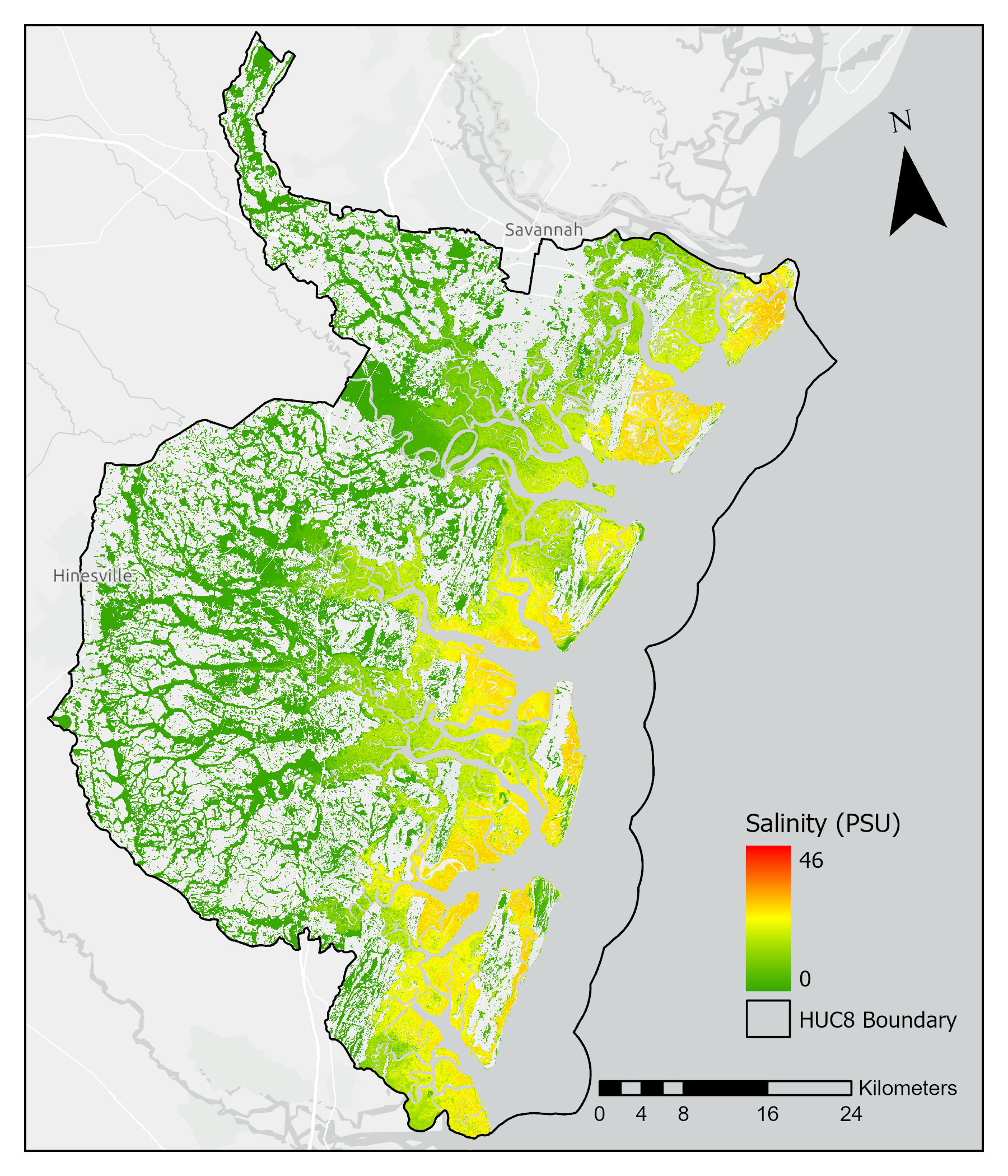
Figure 1. Salinity modeled in practical salinity units to the Sapelo Island National Estuarine Research Reserve watershed in coastal Georgia, U.S.
Citation
Holmquist, J.R., and A. Carr. 2025. Wetland Salinity Maps of Select Estuary Sites in the United States, 2020. ORNL DAAC, Oak Ridge, Tennessee, USA. https://doi.org/10.3334/ORNLDAAC/2392
Table of Contents
- Dataset Overview
- Data Characteristics
- Application and Derivation
- Quality Assessment
- Data Acquisition, Materials, and Methods
- Data Access
- References
Dataset Overview
This dataset provides gridded average annual wetland salinity concentrations in practical salinity units (PSU) at 30-meter resolution within 24 coastal estuary sites in the United States predicted for 2020. Salinity in estuaries can serve as a proxy for sulfate concentration, which can inhibit methanogenesis. Data were derived from a hybrid approach to mapping salinity as a continuous variable using a combination of physical watershed and stream characteristics, optical remote sensing based on vegetation characteristics, and climate variables. Data are provided in cloud-optimized GeoTIFF format covering 33 Hydrologic Unit Code 8-digit (HUC8) watersheds to the extent of palustrine and estuarine wetlands as defined by NOAA's 2016 Coastal Change Analysis Program (C-CAP) Coastal Land Cover layer. Additionally, model outputs are provided in comma separated values (CSV) files, and code scripts are provided in a compressed (*.zip) file.
Project: Carbon Monitoring System
The NASA Carbon Monitoring System (CMS) is designed to make significant contributions in characterizing, quantifying, understanding, and predicting the evolution of global carbon sources and sinks through improved monitoring of carbon stocks and fluxes. The System will use the full range of NASA satellite observations and modeling/analysis capabilities to establish the accuracy, quantitative uncertainties, and utility of products for supporting national and international policy, regulatory, and management activities. CMS will maintain a global emphasis while providing finer scale regional information, utilizing space-based and surface-based data and will rapidly initiate generation and distribution of products both for user evaluation and to inform near-term policy development and planning.
Acknowledgment:
This Carbon Monitoring Systems project was supported primarily by NASA's Carbon Monitoring System program (grant 80NSSC20K0084).
Data Characteristics
Spatial Coverage: Tidal wetlands within the contiguous United States
Spatial Resolution: 30 m
Temporal Coverage: 2020-01-01 to 2020-12-31
Temporal Resolution: One-time estimate
Study Areas: Latitude and longitude are given in decimal degrees.
| Site | Westernmost Longitude | Easternmost Longitude | Northernmost Latitude | Southernmost Latitude |
|---|---|---|---|---|
| Conterminous United States | -124.71 | -69.47 | 48.81 | 26.32 |
Data File Information
This dataset includes 33 cloud-optimized GeoTIFF (*.tif) files of modeled salinity rasters, three comma separated values (*.csv) files of model outputs, and one compressed (*.zip) file of code scripts.
GeoTIFF modeled salinity rasters
There are 33 modeled salinity rasters representing 24 sites in units of practical salinity units for the year 2020 (Table 5). Each file covers one HUC8 watershed to the extent of palustrine and estuarine wetlands as defined by NOAA’s 2016 Coastal Change Analysis Program (C-CAP) Coastal Land Cover layer. Each raster consists of a single band, which represents modeled salinity in units of practical salinity units (PSU, grams salt per 1000 grams water). Pixels not identified as wetlands are assigned a numeric value of -9999.
Files are named: salinity_HUC8_2020_psu.tif; where HUC8 is the 8-digit HUC8 identifier. They have these characteristics:
- Projection: NAD83 / Conus Albers (EPSG: 5070)
- No data value: -9999
- Bands: 1
- Map units: Meters
- Spatial resolution: 30 m
Comma separated values (CSV) files
model_variable_importance.csv contains the ranked importance of the final predictors used in the model.
salinity_predictions_vs_observations.csv is a compilation of observed salinity and model predictions, including residuals, and calibration and validation specific root mean square error and R-squared.
salinity_sampled_calibration_validation_2020.csv holds model training and testing data sampled to all initially determined predictors.
Missing values are represented by ‘-9999’.
Table 1. Data dictionary for model_variable_importance.csv
| Variable | Units | Description |
|---|---|---|
| Variable | - | Predictor variable name |
| Importance | - | Relative importance of variable in the machine learning model\ |
Table 2. Data dictionary for salinity_predictions_vs_observations.csv
| Variable | Units | Description |
|---|---|---|
| Index | - | Row number |
| Predicted_salinity_psu | PSU | Model-predicted practical salinity units (PSU): (g salt) / (kg water) |
| Observed_salinity_psu | PSU | Observed practical salinity units |
| Calibration_or_validation | - | Whether the observation was used for model calibration or training |
| Rmse | PSU | Root-mean square error of predicted versus observed linear regression. |
| Rsquare | 1 | R2, or fraction of total variance explained, by predicted versus observed linear regression. |
| Residual | PSU | Residual variance of predicted versus observed linear regression. |
Table 3. Data dictionary for salinity_sampled_calibration_validation_2020.csv.
| Variable | Units | Description |
|---|---|---|
| Index | Row number | |
| Pathlength | m | Upstream distance (m) |
| Avg_annual_pr_gridmet | mm | Average annual precipitation (mm) |
| Avg_annual_t_gridmet | K | Average annual temperature in degrees Kelvin |
| Blue | 1 | Surface reflectance (0.452-0.512 μm Landsat, 496.6nm (S2A) / 492.1nm (S2B) Sentinel) |
| Elevation_3dep | m | Elevation (m) |
| Evi | 1 | Enhanced Vegetation Index (EVI) |
| Green | 1 | Surface reflectance (SR) (0.533-0.590 μm Landsat, 560nm (S2A) / 559nm (S2B) Sentinel) |
| Nir | 1 | Near infrared surface reflectance (0.851-0.879 μm Landsat, 835.1nm (S2A) / 833nm (S2B) Sentinel) |
| Peak_evi | 1 | Maximum EVI for pixel in 2020 |
| Red | 1 | Surface reflectance (0.636-0.673 μm Landsat, 664.5nm (S2A) / 665nm (S2B) Sentinel) |
| Savi | 1 | Soil Adjusted Vegetation Index |
| Sal_mean_mouth | PSU | Salinity at the mouth of the network in PSU |
| Slope_3dep | Slope (unitless) | |
| Swir1 | 1 | Shortwave Infrared 1 SR (1.566-1.651 μm Landsat, 1613.7nm (S2A) / 1610.4nm (S2B) Sentinel) |
| Swir2 | 1 | Shortwave Infrared 2 SR (2.107-2.294 μm Landsat, 2202.4nm (S2A) / 2185.7nm (S2B) Sentinel) |
| Tbvi_gb | 1 | Two-Band Vegetation Index (Green-Blu) |
| Tbvi_rb | 1 | Two-Band Vegetation Index (Red-Blue) |
| Tbvi_rg | 1 | Two-Band Vegetation Index (Red-Green) |
| Tidal_amp_kriged_mouth | m | Tidal Amplitude at Network Outlet (m) |
| Totdasqkm_mouth | km2 | Total drainage area at Network Outlet (km2) |
| Wdrvi_2 | 1 | Wide Dynamic Range Vegetation Index (0.2) |
| Wdrvi_5 | 1 | Wide Dynamic Range Vegetation Index (0.5) |
| Source | - | Code indicating the source that the data point originated from. |
| Gauge_id | - | Unique identifier indicating unique sampling locations. |
| Gauge_type | - | Code indicating the type of measurement, surface water, marsh well, or porewater sample. |
| Observed_salinity_psu | PSU | Observed practical salinity units |
| Year | YYYY | Year of aggregation. |
| Sd | PSU | Standard deviation of practical salinity units summarized as an annual average. |
| N | 1 | Number of observations summarized as an annual average. |
| Longitude | degrees_east | Longitude in decimal degrees |
| Latitude | degrees_north | Latitude in decimal degrees |
| Watershed | - | Watershed name |
| States | - | US states inside boundary |
| Calibration_or_validation | - | Whether the observation was used for model calibration or training |
| Watershed_left_out | - | Whether the total watershed was left out of the calibration data |
| Index_left_out | - | Whether the individual sampling location was left out of the calibration data |
Code Scripts (*.zip)
There is one compressed (*.zip) file, salinity_scripts_2020.zip, containing R, Google Earth Engine (GEE), and Python (converted from ArcGIS Pro Model Builder) scripts used to develop the GeoTIFF and CSV files. For details on the contents and structure, please see README.txt, which is included inside the compressed file.
Application and Derivation
Coastal wetlands can store carbon and emit methane, and restoration efforts are also capable of reducing their emissions (Holmquist et al., 2018). The effect of uncertainty of palustrine and estuarine methane emissions on the National Greenhouse Gas Inventory (NGGI) is particularly high, so methane mapping is an important step towards improved forecasting. This dataset utilized a geographically diverse synthesis of salinity, because it is much more readily observed than sulfate or methane directly, to model salinity conditions with the intent of deriving improved methane quantifications.
Quality Assessment
The synthesis dataset was partitioned such that approximately 80% (1,376 observations) were used in model calibration, while the remaining data (323) was withheld. Ten percent of the total HUC8 watersheds, and 10% of the total points were randomly selected to be validation data and used to assess the effects of the proximity of calibration data on validation statistics. This assessment produced a root mean square error (RMSE) on the validation subset of 4.94 PSU. The linear regression between the observed and predicted salinity values of the validation subset produced a coefficient of determination (R2) value of 0.764.
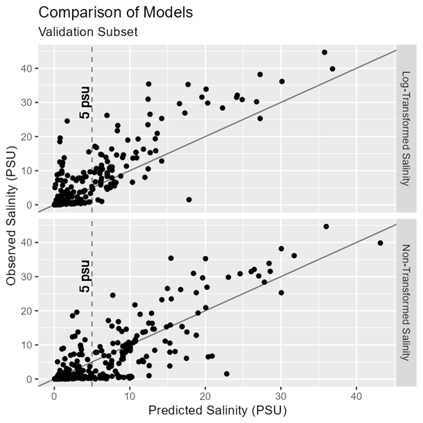
Figure 2. Validation subset predictions compared against observed salinity (PSU) for the random forest model with and without logarithmic transformations applied to select predictors. Lines represent a perfect 1:1 ratio.
The decision to apply the log-transformation to the salinity response variable, salinity kriged to tidal amplitude, and total drainage area produced a trade-off between overall model performance and model performance across the range of salinity most important for methane predictions. The model without the log transformations performed better; the RMSE of the validation subset decreased from 4.94 to 4.76. Model improvements were mixed as R2 decreased from 0.764 to 0.709 for the non-log transformed version. When binning RMSE by 1 psu increments, the log-transformed model performed better across the lowest salinity concentrations (Figure 3). At or below 10 PSU, the RMSE of the log-transformed model was 2.31 PSU compared to 3.79 PSU in the non-log transformed model (Figure 3). Because methane emissions sharply increase between mesohaline (18 to 5 PSU) and oligohaline (0.5 to 5 PSU) salinities and are virtually non-existent at or above 18 PSU (IPCC, 2014), precision below 18 PSU, especially below 5 PSU, is vital. Given mixed model performance and the importance of low-salinity predictions, the log-transformed algorithm was utilized to prioritize accurately mapping the important 5 PSU transitional zone over predicting a broader range of salinities.
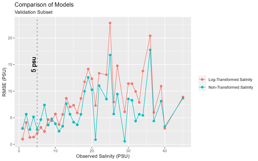
Figure 3. Model performance, indicated by the RMSE between observed salinity and predicted salinity in 1 PSU bin increments, with and without select logarithmically transformed predictors.
Independent validation also showed that the algorithm slightly under-predicted salinity relative to observations (Figure 2). This may be because the calibration dataset was skewed towards low-concentration observations (Figure 4). There were also limited ocean salinity observations (2,383 observations) available to krige oceanic salinity to stream mouths and limited quantity and dispersal along the Pacific coast.
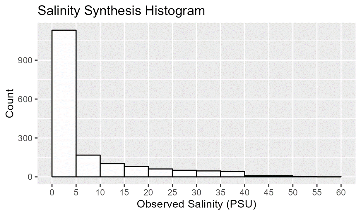
Figure 4. Most synthesized salinity observations were under 5 practical salinity units (PSU).
Data Acquisition, Materials, and Methods
The workflow for assembling the calibration and validation data, as well as generating the remote sensing products is summarized in Figure 5.
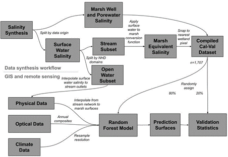
Figure 5. Summary of steps of data synthesis and remote sensing and GIS workflow.
Observations of porewater, marsh well, and surface water surface salinity were synthesized from multiple sources for the purpose of model calibration and validation (Figure 5). These observations were sourced from the following sources: a synthesis of disaggregated porewater measurements by Arias-Ortiz et al. (2024b); the Chesapeake Bay Interpretive Buoy System (CBIBS) (NOAA, 2024b); the Louisiana Coastwide Reference Monitoring system (CPRA, 2024); a porewater sampling campaign by Koontz et. al. (2024); data from Krauss et al. (2016); the National Oceanic and Atmospheric Association’s Physical Oceanic Data (NOAA, 2024a), National Data Buoy Center (NDBC) (NOAA, 2023), and the National Estuarine Research Reserve System (NERRS, 2024) System-wide Monitoring Program (SWMP) (2024); the US Geological Survey’s (USGS) National Water Information System (NWIS) (USGS 1994), queried for salinity and conductivity data, and a regular water quality sampling cruise of San Francisco Bay (Schraga and Cloern, 2017); the Global Change Research Wetland (GCREW) (Cheng et al., 2024a, 2024b; Megonigal et al., 2024); Wilson et al. (2015); and the Environmental Protection Agencies (EPAs) Water Quality Portal (EPA 2013).
All observations were assigned dates and times, positional information (latitude and longitude), and were assigned unique identifiers for the data source of origin, the study of origin for data sources, which synthesized multiple studies, and the type of observation (porewater, marsh well measurement, or surface water). Any conductivity measurements were used to estimate salinity equivalents in PSU using the USGS Coastal Salinity Index R package (McCloskey, 2024). All time-series were simplified to single values per discrete spatial sampling point, mean annual salinities. The number of individual observations was recorded.
Data points were analyzed separately based on their origin (Figure 5). Data from marsh porewater draws, and loggers within wells were added to the calibration and validation dataset without modification and amounted to 1,699 observations. Surface water salinity measurements underwent further sorting and treatment.
Surface water data were further sorted into whether they overlapped open water or stream networks based on our GIS analysis (Figure 5). National Hydrology Dataset (NHD) ‘catchment’ polygons (USGS, 2019) were utilized to determine if surface water points were from the open water (ocean or bay), or were from along stream networks. Observations of open water data (n=2,383) were used to create one of the physical layers in the random forest model, salinity at the mouth of the stream network. Surface water data along stream networks were further treated so that they were equivalent in value and position to marsh data and were used as response data.
For surface water used as response data, extra transformation was used to estimate marsh equivalent salinity from open water salinity and to adjust latitude and longitude from open water to the nearest mapped wetland (Figure 5). First, marsh equivalent salinity was estimated from adjacent open water salinity based on a subset of paired marsh surface well or porewater and surface water observations in the database and a linear regression. Both values were log-transformed. Overall marsh salinity tended to have slightly higher, and less variable, salinity compared to adjacent open water (Figure 6).
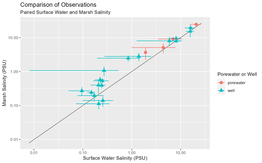
Figure 6. A linear regression model was fit to adjacent surface and marsh salinity observations to derive marsh salinity concentrations from nearby surface observations.
Next, surface observations were snapped to their nearest wetland pixel according to the Coastal Change Analysis Program (C-CAP) (NOAA, 2016) converting given a distance threshold of 90 to 120 m (Figure 5). Open water observations were paired with C-CAP wetlands, which were a maximum of 120 m away (four 30 m pixel widths), to ensure that the inferred wetland observation was associated with the true surface water observation. A minimum threshold of 90 m (three pixel-widths) distance was set so that the inferred observations would be more likely to be associated with interior wetlands, and not bias the analysis towards wetland edges.
The calibration-validation dataset was used to train a random forest algorithm that used 22 potential predictors as inputs (Table 4). A hybrid approach was used that consisted of physical GIS layers representing phenomena likely to influence estuary length and salinity, optical remote sensing indices that contain information on plant community and health, and climate variables for temperature and precipitation.
Table 4. The 22 predictor variables originally chosen for consideration.
| Predictor | Description | Index Equation | Included in Model |
|---|---|---|---|
| pathlength | Upstream distance (m) | TRUE | |
| avg_annual_pr_gridmet | Average annual precipitation (mm) | TRUE | |
| avg_annual_t_gridmet | Average annual temperature (K) | TRUE | |
| blue | Surface reflectance (0.452-0.512 μm Landsat, 496.6nm (S2A) / 492.1nm (S2B) Sentinel) | FALSE | |
| elevation_3dep | Elevation (m) | TRUE | |
| evi | Enhanced Vegetation Index | 2.5 * ((NIR - RED) / (NIR + 6 * RED - 7.5 * BLUE + 1)) | |
| green | Surface reflectance (0.533-0.590 μm Landsat, 560nm (S2A) / 559nm (S2B) Sentinel) | TRUE | |
| nir | Near infrared SR (0.851-0.879 μm Landsat, 835.1nm (S2A) / 833nm (S2B) Sentinel) | TRUE | |
| peak_evi | /Maximum EVI for pixel in 2020 | TRUE | |
| red | Surface reflectance (0.636-0.673 μm Landsat, 664.5nm (S2A) / 665nm (S2B) Sentinel) | FALSE | |
| savi | Soil Adjusted Vegetation Index | (NIR - RED) * 1.5 / (NIR + RED + 0.5) | FALSE |
| sal_mean_mouth | Salinity at the mouth of the network in PSU | TRUE | |
| slope_3dep | /Slope (unitless) | TRUE | |
| swir1 | Shortwave Infrared 1 SR (1.566-1.651 μm Landsat, 1613.7nm (S2A) / 1610.4nm (S2B) Sentinel) | FALSE | |
| swir2 | Shortwave Infrared 2 SR (2.107-2.294 μm Landsat, 2202.4nm (S2A) / 2185.7nm (S2B) Sentinel) | TRUE | |
| tbvi_gb | Two-Band Vegetation Index (Green-Blue) | (GREEN - BLUE) / (GREEN + BLUE) | TRUE |
| tbvi_rb | Two-Band Vegetation Index (Red-Blue) | (RED - BLUE) / (RED + BLUE) | TRUE |
| tbvi_rg | Two-Band Vegetation Index (Red-Green) | (RED - GREEN) / (RED + GREEN) | TRUE |
| tidal_amp_kriged_mouth | Tidal Amplitude at Network Outlet (m) | TRUE | |
| totdasqkm_mouth | Total drainage area at Network Outlet | TRUE | |
| wdrvi_2 | Wide Dynamic Range Vegetation ndex (0.2) | ((0.2 * NIR) - RED) / ((0.2 * NIR) + RED) | FALSE |
| wdrvi_5 | Wide Dynamic Range Vegetation Index (0.5) | ((0.5 * NIR) - RED) / ((0.5 * NIR) + RED) | FALSE |
The spatial predictors consisted of oceanic salinity, total drainage area, and tidal amplitude at the mouth of stream networks, and distance upstream. Surface salinity observations from 2020 and intersecting ocean area features as defined by the National Hydrography Dataset (NHD) (USGS, 2019) were taken from a previous salinity synthesis (Figure 5). Tidal amplitude was kriged from a synthesis of 996 National Water Level Observation Network (NWLON) (NOAA, 2024c) and the Coastwide Reference Monitoring System (CRMS) water level observations made between 1970 and 2019 (CPRA, 2024). Outlets were defined as the point of intersection between NHD coastlines and the most downstream flowline in tidal networks. Oceanic salinity and tidal amplitude were then kriged to each outlet and joined to their respective flowline networks in R. Total upstream cumulative drainage area in square kilometers (TotDASqKm) and distance downstream in kilometers (Pathlength) are attributed to each flowline in the NHD. The drainage area of each network’s terminating flowline was joined with upstream flowlines in the network, while distance downstream was instead preserved for each reach. Flowlines were then converted into point features at the midpoint of each reach, interpolated into wetlands via inverse distance weighting in ArcGIS Pro and exported to TIFF format. This step was completed to the extent of C-CAP wetlands within each HUC8 watershed containing a calibration-validation data point.
Slope and elevation in meters were taken from the 3DEP’s LiDAR-based 10-m National Map (USGS, 2020). 3DEP predictors were equivalently resampled from 10-m to the 30-m scale and projection of C-CAP.
Optical predictors were selected based on their importance in modeling tidal marshland aboveground biomass (Byrd et al., 2018), because biomass was hypothesized to correlate with salinity, and that different plant communities could represent distinct hydrologic conditions descriptive of salinity concentrations (Pennings et al., 2005). Surface reflectance and a suite of vegetation indices were retrieved from the Landsat-8 Level 2, Collection 2, Tier 1 OLI ((USGS, 2013) and Sentinel-2 Level-2A MSI (ESA, 2015) image catalogs in GEE. The image catalogs were first harmonized in GEE. This entailed applying cloud and cloud shadow masking, resampling Sentinel-2 resolution to match Landsat, and adjusting Sentinel-2 band values to match Landsat according to Claverie et al. (2018). The two catalogs were merged and specral indices were calculated (Table 4). Then image collections were reduced into a single median composite for all bands and a maximum annual composite for enhanced vegetation index (EVI). Final images were resampled so that they were the equivalent scale and projection of C-CAP.
Average annual precipitation in millimeters and temperature in Kelvin were retrieved from gridMET (Sierra Nevada Research Institute Climatology Lab; SNRI, 2024). Mean annual temperature was taken as the annual average of the daily average minimum and maximum temperature. GridMet annual averages were resampled from 4-km to the 30-m scale and projection of C-CAP. The interpolated spatial predictors were imported into GEE and composited with the optical, other physical, and climate predictors by HUC8, and then sampled to the calibration-validation dataset.
The sampled predictors were reviewed for near zero variance and high correlation using caret, an R package designed for training classification and regression models. Near zero-variance predictors can unproportionally exert excessive influence on the model (Kuhn, 2008). A predictor would be considered zero-variance if its distribution exhibits a percent uniqueness, the proportion of distinct values out of the count of observations, below 10%, and a frequency ratio, the ratio of the most and second most repeated value, exceeding 19, the defaults of caret’s nearZeroVar() function. None of the predictors were found to meet these criteria; however, seven predictors were dropped for being highly correlated (r>0.9). This is useful because the importance of correlated variables may be underreported.
After redundant predictor variables were removed, the model was calibrated, prediction surfaces were created, and variable importances were calculated in GEE (Gorelick et al., 2017) using the smileRandomForest algorithm with 500 trees.
Distance upstream, maximum EVI, elevation, salinity at network outlets, and average annual temperature were, in order, the top five most important predictors (Fig. 7). Slope had the lowest score and was substantially lower than the next lowest scoring predictor. The model was then used to classify wetlands within the 33 HUC8 watersheds (Table 5). This produced a single-band raster in TIFF format for each HUC8 in which salinity is presented in PSU. Pixels outside of C-CAP wetlands are assigned a numeric value of -9999.
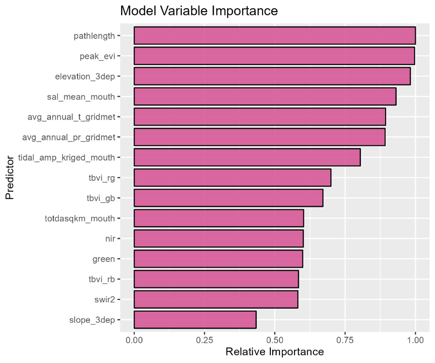
Figure 7. Variable importance of the model’s final predictors relative to the highest scoring variable.
Table 5. Key between HUC8 codes and sites.
| Site Name | HUC8 Code |
|---|---|
| Apalachicola | 03130014 |
| Apalachicola | 03130011 |
| Atchafalaya | 08080101 |
| Atchafalaya | 08090302 |
| Blackbird Creek Reserve | 02040205 |
| /Chesapeake Bay, Virginia | 02080106 |
| Chesapeake Bay, Virginia | 02080107 |
| Chesapeake Bay, Virginia | 02080108 |
| Eden Landing | 18050004 |
| Elkhorn Slough | 18060015 |
| Grand Bay | 03170009 |
| Great Bay | 01060003 |
| Guana Tolomato Matanzas | 03080201 |
| Gulf Shores | 03160205 |
| Hudson River | 02020008 |
| Hudson River | 02020006 |
| Jacques Cousteau | 02040301 |
| Jug Bay | 02060006 |
| Mission-Aransas | 12100404 |
| Mission-Aransas | 12100407 |
| Mission-Aransas | 12100405 |
| Mission-Aransas | 12110202 |
| Monie Bay | 02080110 |
| Narragansett Bay | 01090004 |
| North Inlet-Winyah Bay | 03040208 |
| North Inlet-Winyah Bay | 03040207 |
| Rush Ranch | 18050001 |
| Sapelo Island | 03060204 |
| Smithsonian Environmental Research Center | 02060004 |
| South Slough | 17100304 |
| St. Jones Reserve | 02040207 |
| Tijuana River | 18070305 |
| Waquoit Bay | 01090002 |
Data Access
These data are available through the Oak Ridge National Laboratory (ORNL) Distributed Active Archive Center (DAAC).
Wetland Salinity Maps of Select Estuary Sites in the United States, 2020
Contact for Data Center Access Information:
- E-mail: uso@daac.ornl.gov
- Telephone: +1 (865) 241-3952
References
Arias-Ortiz, A., S.D. Bridgham, J. Holmquist, S. Knox, G. McNicol, B. Needleman, P.Y. Oikawa, E.J. Stuart-Haëntjens, L. Windham-Myers, J. Wolfe, I.C. Anderson, S. Bailey, A. Baldwin, C.E. Bauer, A. Borde, L.J. Brady, P. Brewer, W. Brooks, L. Brophy, J.S. Caplan, M. Capooci, N. Moss Cormier, S. Crooks, V. Cullinan, C.A. Currin, K.M. Czapla, J.W. Day, R. DeLaune, L.A. Deegan, R. Kyle Derby, H. Diefenderfer, B.G. Drake, S.E. Drew, M. Eagle, E.G. Geoghegan, C. Gough, G. Groseclose, C. Gunn, R. Hager, G.O. Holm, T. Hopkins, P.R. Jaffé, C. Janousek, D.J. Johnson, J.K. Keller, C. Kelley, R. Kempka, A. Keshta, H. Kleiner, K.W. Krauss, K.D. Kroeger, R.R. Lane, A. Langley, D.Y. Lee, F.N. Leech, S.K. Mack, M. Madison, A. Mann, J. Marroquin, A.S. Marsh, C. Martens, R. Martin, M. Matsumura, D.E. McWhorter, P. Megonigal, J. Meschter, H.J. Miller, B. Mortazavi, S. Moseman-Valtierra, T.J. Mozdzer, P. Mueller, S.C. Neubauer, S. K Nick, G. Noyce, J. O'Keefe-Suttles, B.C. Perez, H. Poffenbarger, P. Precht, T. Quirk, D.P. Rasse, R.C. Raynie, M. Reid, C. Richardson, B. Roberts, A. Roden, R. Sanders-DeMott, W.H. Schlesinger, M.A. Schultz, C.A. Schutte, K.V. R. Schäfer, J. Shahan, P. Sundareshwar, R. Thom, R. Tripathee, W. Ussler, R. Vargas, D.J. Velinsky, M.A. Vile, P.E. Weber, N.B. Weston, J.L. Whitbeck, B. Wilson, G.E. Woerndle, and S. Yarwood. 2024a. Dataset: Chamber-based Methane Flux Measurements and Other Greenhouse Gas Data for Tidal Wetlands across the Contiguous United States - An Open-Source Database. Smithsonian Environmental Research Center. https://doi.org/10.25573/serc.14227085.v1
Arias-Ortiz, A., J. Wolfe, S.D. Bridgham, S. Knox, G. McNicol, B.A. Needelman, J. Shahan, E.J. Stuart-Haëntjens, L. Windham-Myers, P.Y. Oikawa, D.D. Baldocchi, J.S. Caplan, M. Capooci, K.M. Czapla, R.K. Derby, H.L. Diefenderfer, I. Forbrich, G. Groseclose, J.K. Keller, C. Kelley, A.E. Keshta, H.S. Kleiner, K.W. Krauss, R.R. Lane, S. Mack, S. Moseman-Valtierra, T.J. Mozdzer, P. Mueller, S.C. Neubauer, G. Noyce, K.V. R. Schäfer, R. Sanders-DeMott, C.A. Schutte, R. Vargas, N.B. Weston, B. Wilson, J.P. Megonigal, and J.R. Holmquist. 2024b. Methane fluxes in tidal marshes of the conterminous United States. Global Change Biology 30:e17462. https://doi.org/10.1111/gcb.17462
Byrd, K.B., L. Ballanti, N. Thomas, D. Nguyen, J.R. Holmquist, M. Simard, and L. Windham-Myers. 2018. A remote sensing-based model of tidal marsh aboveground carbon stocks for the conterminous United States. ISPRS Journal of Photogrammetry and Remote Sensing 139:255–271. https://doi.org/10.1016/j.isprsjprs.2018.03.019
Cheng, S., G. Noyce, P. Megonigal, and R. Rich. 2024a. 2017-2024 L0 SMARTX C3 Water Level and Salinity Record, Smithsonian Environmental Research Center. Smithsonian Environmental Research Center. https://doi.org/10.25573/serc.27835395.v1
Cheng, S., G. Noyce, P. Megonigal, and R. Rich. 2024b. 2017-2024 L0 SMARTX C4 Water Level and Salinity Record, Smithsonian Environmental Research Center. Smithsonian Environmental Research Center. https://doi.org/10.25573/serc.27868569.v2
Claverie, M., J. Ju, J.G. Masek, J.L. Dungan, E.F. Vermote, J.-C. Roger, S.V. Skakun, and C. Justice. 2018. The Harmonized Landsat and Sentinel-2 surface reflectance data set. Remote Sensing of Environment 219:145–161. https://doi.org/10.1016/j.rse.2018.09.002
Coastal Protection and Restoration Authority (CPRA) of Louisiana. 2024. Coastwide Reference Monitoring System-Wetlands Monitoring Data. http://cims.coastal.louisiana.gov
Environmental Protection Agency (EPA) and United States Geological Survey. 2013. Water Quality Portal. U.S. Geological Survey. https://doi.org/10.5066/P9QRKUVJ
European Space Agency (ESA). 2015. Sentinel-2 MSI Level-2A BOA Reflectance. https://doi.org/10.5270/S2_-6eb6imz
Gorelick, N., M. Hancher, M. Dixon, S. Ilyushchenko, D. Thau, and R. Moore. 2017. Google Earth Engine: Planetary-scale geospatial analysis for everyone. Remote Sensing of Environment 202:18–27. https://doi.org/10.1016/j.rse.2017.06.031
Holmquist, J.R., L. Windham-Myers, B. Bernal, K.B. Byrd, S. Crooks, M.E. Gonneea, N. Herold, S.H. Knox, K.D. Kroeger, J. McCombs, J.P. Megonigal, M. Lu, J.T. Morris, A.E. Sutton-Grier, T.G. Troxler, and D.E. Weller. 2018. Uncertainty in United States coastal wetland greenhouse gas inventorying. Environmental Research Letters 13:115005. https://doi.org/10.1088/1748-9326/aae157
IPCC 2014, 2013 Supplement to the 2006 IPCC Guidelines for National Greenhouse Gas Inventories: Wetlands, Hiraishi, T., Krug, T., Tanabe, K., Srivastava, N., Baasansuren, J., Fukuda, M. and Troxler, T.G. (eds). Published: IPCC, Switzerland. https://www.ipcc.ch/site/assets/uploads/2018/03/Wetlands_Supplement_Entire_Report.pdf
Koontz, E.L., S.M. Parker, A.E. Stearns, B.J. Roberts, C.M. Young, L. Windham-Myers, P.Y. Oikawa, J.P. Megonigal, G.L. Noyce, E.J. Buskey, R.K. Derby, R.P. Dunn, M.C. Ferner, J.L. Krask, C.M. Marconi, K.B. Savage, J. Shahan, A.C. Spivak, K.A. St. Laurent, J.M. Argueta, S.J. Baird, K.M. Beheshti, L.C. Crane, K.A. Cressman, J.A. Crooks, S.H. Fernald, J.A. Garwood, J.S. Goldstein, T.M. Grothues, A. Habeck, S.B. Lerberg, S.B. Lucas, P. Marcum, C.R. Peter, S.W. Phipps, K.B. Raposa, A.S. Rovai, S.S. Schooler, R.R. Twilley, M.C. Tyrrell, K.A. Uyeda, S.H. Wulfing, J.T. Aman, A. Giacchetti, S.N. Cross-Johnson, and J.R. Holmquist. 2024. Controls on spatial variation in porewater methane concentrations across United States tidal wetlands. Science of The Total Environment 957:177290. https://doi.org/10.1016/j.scitotenv.2024.177290
Krauss, K.W., G.O. Holm, B.C. Perez, D.E. McWhorter, N. Cormier, R.F. Moss, D.J. Johnson, S.C. Neubauer, and R.C. Raynie. 2016. Component greenhouse gas fluxes and radiative balance from two deltaic marshes in Louisiana: Pairing chamber techniques and eddy covariance. Journal of Geophysical Research: Biogeosciences 121:1503–1521. https://doi.org/10.1002/2015JG003224
Kuhn, M. 2008. Building Predictive Models in R Using the caret Package. Journal of Statistical Software 28:1-26. https://doi.org/10.18637/jss.v028.i05
McCloskey, B. 2024. CSI: Coastal Salinity Index. R package version 0.0.1. https://github.com/USGS-R/CSI
Megonigal, J.P., M.E. Hines, and P.T. Visscher. 2004. Anaerobic Metabolism: Linkages to Trace Gases and Aerobic Processes. Treatise on Geochemistry:317–424. https://doi.org/10.1016/B0-08-043751-6/08132-9
Megonigal, P., A. Peresta, P. Neale, R. Rich, S. Cheng, and A. Tashjian. 2024. 2018-2024 L0 Water Quality Data from Marsh Outlet Exo Sonde, Smithsonian Environmental Research Center. Smithsonian Environmental Research Center. https://doi.org/10.25573/serc.27871395.v1
National Atomospheric and Oceanic Administration (NOAA). 2024a. Physical Oceanography Data. https://tidesandcurrents.noaa.gov/stations.html?type=Physical%20Oceanography
National Oceanic and Atmospheric Administration (NOAA). 2016. C-CAP 1996-2010-Era Land Cover Change Data. https://coast.noaa.gov/digitalcoast/data/ccapregional.html
National Oceanic and Atmospheric Administration (NOAA). 2023. National Data Buoy Center. http://ndbc.noaa.gov/data
National Oceanic and Atmospheric Administration (NOAA). 2024b. Chesapeake Bay Interpretive Buoy System. https://buoybay.noaa.gov/data
National Oceanic and Atmospheric Administration (NOAA). 2024c. National Water Level Observation Network (NWLON). Retrieved from Center for Operational Oceanographic Products and Services (CO-OPS) database. https://tidesandcurrents.noaa.gov/nwlon.html
NOAA National Estuarine Research Reserve System (NERRS). 2024. System-wide Monitoring Program. http://www.nerrsdata.org
Pennings, S.C., M. Grant, and M.D. Bertness. 2004. Plant zonation in lowa's latitude salt marshes: disentangling the roles of flooding, salinity and competition. Journal of Ecology 93:159–167. https://doi.org/10.1111/j.1365-2745.2004.00959.x
Schraga, T.S., and J.E. Cloern. 2017. Water quality measurements in San Francisco Bay by the U.S. Geological Survey, 1969–2015. Scientific Data 4. https://doi.org/10.1038/sdata.2017.98
Sierra Nevada Research Institute (SNRI) Climatology Lab. 2024. Gridded Surface Meteorological (gridMET) Dataset. https://developers.google.com/earth-engine/datasets/catalog/IDAHO_EPSCOR_GRIDMET
United States Geological Survey (USGS). 1994. USGS Water Data for the Nation. U.S. Geological Survey. https://doi.org/10.5066/F7P55KJN
U.S. Geological Survey (USGS) Earth Resources Observation and Science (EROS) Center. 2013. Landsat 8-9 Operational Land Imager / Thermal Infrared Sensor Level-2, Collection 2. U.S. Geological Survey. https://doi.org/10.5066/P9OGBGM6
U.S. Geological Survey (USGS). 2019. National Hydrography Dataset Plus (NHDPlus) High Resolution V21. https://www.usgs.gov/national-hydrography/access-national-hydrography-products
U.S. Geological Survey (USGS). 2020. 3D Elevation Program (3DEP) 10m National Map Seamless (1/3 Arc-Second). https://developers.google.com/earth-engine/datasets/catalog/USGS_3DEP_10m
Wilson, B.J., B. Mortazavi, and R.P. Kiene. 2015. Spatial and temporal variability in carbon dioxide and methane exchange at three coastal marshes along a salinity gradient in a northern Gulf of Mexico estuary. Biogeochemistry 123:329–347. https://doi.org/10.1007/s10533-015-0085-4