Documentation Revision Date: 2020-09-24
Dataset Version: 1
Summary
The Bayesian framework required the development of Light Use Efficiency (LUE) equations specific to tidal wetland classes and the optimal values of a set of characteristics that quantify the controls of light and temperature on EC-derived GPP. The EC tower datasets spanned multiple years across all seasons and the full range of possible light and temperature controls. The model was validated by comparing its predicted GPP with GPP from the 10 EC tower sites. After validation, GPP was mapped across tidal wetlands at 16-day intervals. Daily average per m2 GPP was calculated within individual tidal wetland pixels. The predicted GPP by wetland class was multiplied by the percent cover of each class in the pixel for the woody and herbaceous classes separately, and then the two were summed to find the GPP in each pixel.
There are 454 data files in GeoTIFF (.tif) format at 250 m spatial resolution. This includes 453 files for tidal wetland gross primary production (GPP) at 16-day intervals beginning March 5, 2000, through November 1, 2019. There is one file that describes the tidal wetland area of each pixel.
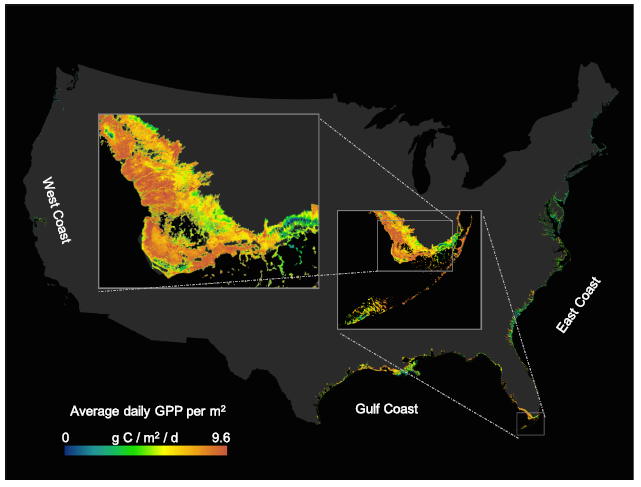
Figure 1. Example of average daily gross primary production (GPP) per m2 at 250 m resolution shown for wetlands in the North and South Ten Thousand Islands in the Florida Everglades. Mapped values are an average of all 16-day periods from 2000-2019. Source: Feagin et al., 2020
Citation
Feagin, R.A., I. Forbrich, T.P. Huff, J.G. Barr, J. Ruiz-plancarte, J.D Fuentes, R.G. Najjar, R. Vargas, A. Vazquez-lule, L. Windham-Myers, K. Kroeger, E.J. Ward, G.W. Moore, M. Leclerc, K.W. Krauss, C.L. Stagg, M. Alber, S.H. Knox, K.V.R. Schafer, T.S. Bianchi, J.A. Hutchings, H.B. Nahrawi, A. Noormets, B. Mitra, A. Jaimes, A.L. Hinson, B. Bergamaschi, J. King, and G. Miao. 2020. Gross Primary Production Maps of Tidal Wetlands across Conterminous USA, 2000-2019. ORNL DAAC, Oak Ridge, Tennessee, USA. https://doi.org/10.3334/ORNLDAAC/1792
Table of Contents
- Dataset Overview
- Data Characteristics
- Application and Derivation
- Quality Assessment
- Data Acquisition, Materials, and Methods
- Data Access
- References
Dataset Overview
This dataset provides mapped tidal wetland gross primary production (GPP) estimates (g C/m2/day) derived from multiple wetland types at 250 m resolution across the conterminous United States at 16-day intervals from March 5, 2000, through November 17, 2019. GPP was derived with the spatially explicit Blue Carbon (BC) model, which combined tidal wetland cover and field-based eddy covariance (EC) tower GPP data into a single Bayesian framework and the Moderate Resolution Imaging Spectroradiometer (MODIS) Enhanced Vegetation Index (EVI). Model development entailed determining the locations of and grouping of tidal wetlands into four classes: woody mangroves, woody freshwater swamps, herbaceous salt marshes, and herbaceous freshwater wetlands. Tidal wetlands are a critical component of global climate regulation. Tidal wetland-based carbon, or "blue carbon," is a valued resource that is increasingly important for restoration and conservation purposes.
The Bayesian framework required the development of Light Use Efficiency (LUE) equations specific to tidal wetland classes and the optimal values of a set of characteristics that quantify the controls of light and temperature on EC-derived GPP. The EC tower data sets spanned multiple years across all seasons and the full range of possible light and temperature controls. The model was validated by comparing its predicted GPP with GPP from the 10 EC tower sites. After validation, GPP was mapped across tidal wetlands at 16-day intervals. Daily average per m2 GPP was calculated within individual tidal wetland pixels. The predicted GPP by wetland class was multiplied by the percent cover of each class in the pixel for the woody and herbaceous classes separately, and then the two were summed to find the GPP in each pixel.
Project: Carbon Monitoring System
The NASA Carbon Monitoring System (CMS) is designed to make significant contributions in characterizing, quantifying, understanding, and predicting the evolution of global carbon sources and sinks through improved monitoring of carbon stocks and fluxes. The System will use the full range of NASA satellite observations and modeling/analysis capabilities to establish the accuracy, quantitative uncertainties, and utility of products for supporting national and international policy, regulatory, and management activities. CMS will maintain a global emphasis while providing finer scale regional information, utilizing space-based and surface-based data and will rapidly initiate generation and distribution of products both for user evaluation and to inform near-term policy development and planning.
Related Publications
Feagin, R.A., Forbrich, I., Huff, T.P., Barr, J.G., Ruiz-Plancarte, J., Fuentes, J.D., Najjar, R.G., Vargas, R., Vázquez-Lule, A.L., Windham-Myers, L., Kroeger, K.D., Ward, E.J., Moore, G.W., Leclerc, M., Krauss, K.W., Stagg, C.L., Alber, M., Knox, S.H., Schäfer, K.V.R., Bianchi, T.S., Hutchings, J.A., Nahrawi, H., Noormets, A., Mitra, B., Miao, G., Jaimes, A., Hinson, A.L., Bergamaschi, B., King J.S. 2020. Tidal wetland Gross Primary Production (GPP) across the continental United States, 2000-2019. Global Biogeochemical Cycles 34: e2019GB006349. https://doi.org/10.1029/2019GB006349
Related Datasets
Summary data files, model codes, and other resources are publicly available at bluecarbon.tamu.edu. The authors encourage others to explore and use the BC model and maps to make new discoveries about tidal wetland GPP.
Holmquist, J.R., L. Windham-Myers, N. Bliss, S. Crooks, J.T. Morris, P.J. Megonigal, T. Troxler, D. Weller, J. Callaway, J. Drexler, M.C. Ferner, M.E. Gonneea, K. Kroeger, L. Schile-beers, I. Woo, K. Buffington, B.M. Boyd, J. Breithaupt, L.N. Brown, N. Dix, L. Hice, B.P. Horton, G.M. Macdonald, R.P. Moyer, W. Reay, T. Shaw, E. Smith, J.M. Smoak, C. Sommerfield, K. Thorne, D. Velinsky, E. Watson, K. Grimes, and M. Woodrey. 2019. Tidal Wetland Soil Carbon Stocks for the Conterminous United States, 2006-2010. ORNL DAAC, Oak Ridge, Tennessee, USA. https://doi.org/10.3334/ORNLDAAC/1612
Byrd, K.B., L. Ballanti, N. Thomas, D. Nguyen, J.R. Holmquist, M. Simard, and L. Windham-Myers. 2018. Aboveground Biomass High-Resolution Maps for Selected US Tidal Marshes, 2015. ORNL DAAC, Oak Ridge, Tennessee, USA. https://doi.org/10.3334/ORNLDAAC/1610
Ballanti, L., and K.B. Byrd. 2018. Vegetation and Open Water High-Resolution Maps for Selected US Tidal Marshes, 2015. ORNL DAAC, Oak Ridge, Tennessee, USA. https://doi.org/10.3334/ORNLDAAC/1609
Ballanti, L., and K.B. Byrd. 2018. Green Vegetation Fraction High-Resolution Maps for Selected US Tidal Marshes, 2015. ORNL DAAC, Oak Ridge, Tennessee, USA. https://doi.org/10.3334/ORNLDAAC/1608
Acknowledgment
This work was funded by NASA Carbon Monitoring System (CMS) Program (grants NNX14AM37G and NNH14AY671).
Data Characteristics
Spatial Coverage: Tidal wetlands across the conterminous United States
Spatial Resolution: 250 m
Temporal Coverage: 2000-03-05 to 2019-11-17
Temporal Resolution: 16-day interval
Study Area: Latitude and longitude are given in decimal degrees.
| Sites | Westernmost Longitude | Easternmost Longitude | Northernmost Latitude | Southernmost Latitude |
|---|---|---|---|---|
| Continental US | -128.0256 | -65.9019 | 47.69669 | 23.50166 |
Data File Information
There are 454 data files in GeoTIFF (.tif) format at 250 m spatial resolution. This includes 453 files for tidal wetland gross primary production (GPP) at 16-day intervals from March 5, 2000, to November 1, 2019. There is one file that describes the tidal wetland area of each pixel.
Table 1. Data file names and descriptions.
| File names | Units | Description |
|---|---|---|
| tidal_wetland_GPP_YYYY_MM_DD.tif | gC/m2/d |
Gross primary production (GPP) in grams of carbon per square meter per day, where YYYY = 2000-2019, MM = month, DD = day. The data files are proved at 16-day intervals beginning March 5, 2000, with the last file dated November 1, 2019. |
| area_of_tidal_wetlands.tif | m2 | Tidal wetland area within each 250 m resolution pixel. |
Data File Details
For each GeoTIFF file,
Projection: WGS 84 / UTM zone 14N, EPSG:32614
Map units: meter
No data value: -9999
Application and Derivation
Tidal wetlands are a critical component of global climate regulation. Their GPP represents the total photosynthetic flux of CO2 between the atmosphere and the surface on a per land area basis before any respiratory fluxes back to the atmosphere are removed. Tidal wetland-based carbon, or "blue carbon," is a valued resource that is increasingly important for restoration and conservation purposes.
If a user wants to aggregate or sum the total tidal wetland GPP within or across pixels, then multiply the average GPP by the area of tidal wetlands within each pixel using the data files provided.
Quality Assessment
Uncertainty and accuracy of the data were assessed in several ways. First, the BC model data were checked against field-derived EC GPP data at 10 sites around the US; it produced an RMSE of 1.22 g C/m2/day, with an average error at 7% with a mean bias of nearly zero. An internal interpolation procedure was assessed to have induced approximately 2.2% of this total error. The data were also checked against other related datasets and heuristic calculations for consistency. More details on uncertainty and error can be found in the associated publication by Feagin et al. (2020).
Data Acquisition, Materials, and Methods
GPP was estimated with the spatially-explicit BC model, which combined tidal wetland cover and field-based EC tower data into a single Bayesian framework, and used a supercomputer network and remote sensing imagery (i.e. MODIS EVI; Didan 2015). The BC model also included mixed pixels in areas not covered by MOD17 GPP product (Running et al., 2015), which comprised approximately 16.8% of tidal wetland GPP. The model approach applied seven basic steps, illustrated in Figure 2.
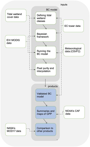
Figure 2. Overview of the input datasets, processes, and products of the BC model. Source: Feagin et al., 2020
Description of the steps in Figure 2
First, specific types of wetlands were defined based on mapping data and EC tower data availability (Table 2). The locations of all tidal wetlands were identified and grouped into four separate classes: (1) woody mangroves, (2) woody freshwater swamps, (3) herbaceous salt marshes, and (4) herbaceous freshwater wetlands. These four classes form a full factorial that includes all tidal wetlands. The resulting high-resolution, resolution, vector-based dataset was composed of polygonal delineations. Hinson et al. (2017) provide more details on the underlying dataset (downloadable from bluecarbon.tamu.edu), which is a refinement of the National Wetlands Inventory and as such, its classification is based on the Cowardin system (Cowardin et al., 1979). In short, the definition of a tidal wetland in this dataset is based on hydrologic considerations which are listed as specific modifiers (e.g., semi-permanently flooded tidal freshwater wetland; Federal Geographic Data Committee, 2019). A MODIS grid was then overlaid on top of this vector data set and the area of each tidal wetland class was determined within a 250 m pixel size. This step allowed the class affiliation to be identified and the percent of each pixel occupied by each class, at the 250 m scale.
Second, to compute estimates of tidal wetland GPP at a given location and date, our approach with the BC model required input for each of the variables outlined in equation 1 below:
 (1)
(1)
For modeling LUE (equation 1), ε required extensive parameterization within a hierarchical Bayesian statistical framework. This framework required the development of LUE equations specific to tidal wetlands and the optimal values of a set of characteristics that quantify the controls of light and temperature on EC-derived GPP. This framework used EC tower datasets at several wetland sites, with datasets spanning multiple years across all seasons (and thus the full range of possible light and temperature controls) (Table 2). Atmospheric fluxes of NEE at the sites were determined using the eddy covariance technique (Baldocchi et al., 1988). The calculated fluxes were either downloaded directly from Ameriflux or provided by site principal investigators. With the exception of US-NC4, all sites experienced tidal hydrology (the hydrology of US-NC4 is classified as “seasonally flooded” in the National Wetlands Inventory).
Third, using the results from the Bayesian framework as the BC model inputs, the BC model then calculated equation (1). The iPAR inputs were derived from meteorological datasets: NCEP Climate Forecast System Version 2 6-hourly products (CFSV2) (Saha et al., 2011), and downward solar radiation flux at 6-hour intervals (imagery layer name in Google Earth Engine: Downward_Short-Wave_Radiation_Flux_surface_6_Hour_Average) (Gorelick et al., 2017). The fPAR inputs were derived from MODIS EVI datasets (MOD13Q1; Didan 2015) at 16-day time intervals and at 250-m spatial resolution across the continental United States.
Fourth, a unique spatial algorithm was developed to solve the problem of “mixed pixels”.
Fifth, the validity of the BC model was assessed by comparing its GPP predictions with field-derived EC tower GPP. The BC model output GPP predictions were compared with field-derived GPP from the 10 EC tower sites (Table 2). For four of the tower locations, some years were used during parameterization of the Bayesian model (designated P in Table 2), while other years were used for validation (designated V and N). For the other six “offsite” locations, all data were used only at the validation stage (designated O). The BC model performance was evaluated using linear regression and standard metrics for goodness-of-fit. After validation of the BC model, GPP was mapped across tidal wetlands at 16-day intervals for the years 2000–2019. Daily average per m2 GPP and total annual GPP were calculated within individual tidal wetland pixels. The predicted GPP by class was multiplied by the percent cover of each class in the pixel for the woody and herbaceous classes separately, and then the two were summed to find the GPP in each pixel.
Sixth, tidal wetland GPP was mapped over the relevant spatiotemporal extent.
Finally, the BC model was compared with NASA's MOD17 GPP product (Feagin et al., 2020; Running et al., 2015).
Table 2. Summary of Flux Datasets Used During Parameterization and Validation of the Bayesian Framework and BC Model.
| EC tower site ID, Name (State) | Location | Example Reference | Dominant Plant Species | BC Model Class | Datesa |
|---|---|---|---|---|---|
| US-SKR, Shark River Slough Everglades (Florida) | 25.363293, −81.077544 | Barr et al. (2013) | Rhizophora mangle, Avicennia germinans, Laguncularia racemosa | Woody (Mangroves) | P 2007–2008 |
| V 2009–2010 | |||||
| N 2004–2006; 2011 | |||||
| US-NC4, Alligator River (North Carolina) | 35.787717, −75.903952 | Miao et al. (2017) | Taxodium distichum, Nyssa aquatica, Acer rubrum | Woody (Freshwater Swamp) | P 2013–2014 |
| V 2015–2016 | |||||
| US-PHM, Plum Island High Marsh (Massachusetts) | 42.742443, −70.830219 | Forbrich et al. (2018) | Spartina patens, Spartina alterniflora, Distichlis spicata | Herbaceous (Salt Marsh) | P 2013–2014 |
| V 2015–2016 | |||||
| N 2017 | |||||
| US-SRR, Suisun Marsh-Rush Ranch (California) | 38.200556, −122.02635 | Knox et al. (2018) | Schoenoplectus spp., Typha spp., Lepidium latifolium L. | Herbaceous (Freshwater Wetland) | P 2014–2015 |
| V 2016–2017 | |||||
| US-PLM, Plum Island Low Marsh (Massachusetts) | 42.734463, −70.838231 | N/A | Spartina alterniflora | Herbaceous (Salt Marsh) | O 2015–2017 |
| US-HPY, Hawk Property (New Jersey) | 40.769173, −74.085318 | Duman and Schäfer (2018) | Spartina patens, Phragmites australis | Herbaceous (Salt Marsh) | O 2014–2017 |
| US-STJ, St. Jones Reserve (Delaware) | 39.088225, −75.437210 | Capooci et al. (2019) | Spartina alterniflora, Spartina cynosuroides | Herbaceous (Salt Marsh) | O 2016–2017 |
| US-VFP, Virginia Coast Res. Following Point (Virginia) | 37.411065, −75.833208 | N/A | Spartina alterniflora | Herbaceous (Salt Marsh) | O 2015–2017 |
| GCE, Georgia Coastal Ecosystems LTER (Georgia) | 31.444094, −81.283444 | Tao et al. (2018) | Spartina alterniflora | Herbaceous (Salt Marsh) | O 2013–2015 |
| US-LA1, Pointe-aux-Chenes Brackish Marsh (Louisiana) | 29.501303, −90.444897 | Krauss et al. (2016) | Spartina patens | Herbaceous (Freshwater Wetland) | O 2012 |
a Codes denote how each year of EC tower field-derived data were used for the final two class model (woody and herbaceous classes): P = parameterization of Bayesian framework only; V = validation for Bayesian framework and BC model; N = validation for BC model use only; O = “offsite” validation for BC model use only. Refer to Feagin et al., 2020 for details.
Data Access
These data are available through the Oak Ridge National Laboratory (ORNL) Distributed Active Archive Center (DAAC).
Gross Primary Production Maps of Tidal Wetlands across Conterminous USA, 2000-2019
Contact for Data Center Access Information:
- E-mail: uso@daac.ornl.gov
- Telephone: +1 (865) 241-3952
References
Baldocchi, D.D., B.B. Hincks, and T.P. Meyers. 1988. Measuring biosphere-atmosphere exchanges of biologically related gases with micrometeorological methods. Ecology, 69, 1331–1340. http://doi.org/10.2307/1941631
Barr, J.G., V. Engel, J.D. Fuentes, D.O. Fuller, and H. Kwon. 2013. Modeling light use efficiency in a subtropical mangrove forest equipped with CO2 eddy covariance. Biogeosciences, 10, 2145–2158. https://doi.org/10.5194/bg-10-2145-2013
Capooci, M., J. Barba, A. Seyfferth, and R. Vargas. 2019. Experimental influence of storm surge salinity on soil greenhouse gas emissions from a tidal marsh. Science of the Total Environment, 686, 1164–1172. https://doi.org/10.1016/j.scitotenv.2019.06.032
Cowardin, L.M., V. Carter, F.C. Golet, and E.T. LaRoe. 1979. Classification of wetlands and deepwater habitats of the United States. US Fish and Wildlife, Report No. FWS/OBS-78/31.
Didan, K. MOD13Q1 MODIS/Terra Vegetation Indices 16-Day L3 Global 250m SIN Grid V006. 2015, distributed by NASA EOSDIS Land Processes DAAC, https://doi.org/10.5067/MODIS/MOD13Q1.006
Duman, T., and K.V.R. Schafer. 2018. Partitioning net ecosystem carbon exchange of native and invasive plant communities by vegetation cover in an urban tidal wetland in the New Jersey Meadowlands (USA). Ecological Engineering, 114, 16–24. https://doi.org/10.1016/j.ecoleng.2017.08.031
Feagin, R.A., I. Forbrich, T.P. Huff, J.G. Barr, J. Ruiz-Plancarte, J.D. Fuentes, R.G. Najjar, R. Vargas, A. Vazquez-Lule, L. Windham-Myers, K.D. Kroeger, E.J. Ward, G.W. Moore, M. Leclerc, K.W. Krauss, C.L. Stagg, M. Alber, S.H. Knox, K.V.R . Schafer, T.S. Bianchi, J.A. Hutchings, H. Nahrawi, A. Noormets, B. Mitra, A. Jaimes, A.L. Hinson, B. Bergamaschi, J.S. King, and G. Miao. 2020. Tidal wetland Gross Primary Production (GPP) across the continental United States, 2000-2019. Global Biogeochemical Cycles 34: e2019GB006349. https://doi.org/ 10.1029/2019GB006349
Federal Geographic Data Committee. 2019. Classification of wetlands and deepwater habitats of the United States. February 2019 version. https://www.fws.gov/wetlands/documents/NWI_Wetlands_and_Deepwater_Map_Code_D
Forbrich, I., A.E. Giblin, and C.S. Hopkinson. 2018. Constraining marsh carbon budgets using long-term C burial and contemporary atmospheric CO2 fluxes. Journal of Geophysical Research: Biogeosciences, 123, 867–878. https://doi.org/10.1002/2017JG004336
Gorelick, N., M. Hancher, M. Dixon, S. Ilyuschchenko, D. Thau, and R. Moore. (2017). Google Earth Engine: Planetary-scale geospatial analysis for everyone. Remote Sensing of the Environment, 202, 18–27. https://doi.org/10.1016/j.rse.2017.06.031
Hinson, A.L., R.A. Feagin, M. Eriksson, R.G. Najjar, M. Herrmann, T.S. Bianchi, M. Kemp, J.A. Hutchings, S. Crooks, and T. Boutton. 2017. The spatial distribution of soil organic carbon in tidal wetland soils of the continental United States. Global Change Biology, 23, 5468–5480. https://doi.org/ 10.1111/gcb.13811
Knox, S.H., L. Windham-Myers, F. Anderson, C. Sturtevant, and B. Bergamaschi. 2018. Direct and indirect effects of tides on ecosystem-scale CO2 exchange in a brackish tidal marsh in Northern California. Journal of Geophysical Research Biogeosciences, 123, 787–806. https://doi.org/10.1002/2017JG004048
Krauss, K.W., G.O. Holm Jr., B.C. Perez, D.E. McWorter, N. Cormier, R.F. Moss, D.J. Johnson, S.C. Neubauer, and R.C. Raynie. 2016. Component greenhouse gas fluxes and radiative balance from two deltaic marshes in Louisiana: Pairing chamber techniques and eddy covariance. Journal of Geophysical Research: Biogeosciences, 121, 1503–1521. https://doi.org/10.1002/2015JG003224
Miao, G., A. Noormets, J.C. Domec, M.F. Fuentes, C.C. Trettin, G. Sun, S.G. McNulty, and J.S. King. 2017. Hydrology and microtopography control carbon dynamics in wetlands: implications in partitioning ecosystem respiration in a coastal plain forested wetland. Agricultural and Forest Meteorology, 247, 343–355. https://doi.org/10.1016/j.agrformet.2017.08.022
Running, S., Q. Mu, M. Zhao. MOD17A2H MODIS/Terra Gross Primary Productivity 8-Day L4 Global 500m SIN Grid V006. 2015, distributed by NASA EOSDIS Land Processes DAAC, https://doi.org/10.5067/MODIS/MOD17A2H.006
Saha, S., S. Moorthi, X. Wu, J. Wang, S. Nadiga, P. Tripp, D. Behringer, Y. Hou, H. Chuang, M. Iredell, M. Ek, J. Meng, R. Yang, M. Mendez, H. van den Dool, Q. Zhang, W. Wang, M. Chen, and E. Becker, 2011, updated daily. NCEP Climate Forecast System Version 2 (CFSv2) 6-hourly Products. Research Data Archive at the National Center for Atmospheric Research, Computational and Information Systems Laboratory. Accessed 14 05 2019. https://doi.org/10.5065/D61C1TXF
Tao, J., D.R. Mishra, D.L. Cotton, J. O'Connell, M. Leclerc, H. Binti Nahrawi, G. Zhang, and R. Pahari. 2018. A comparison between the MODIS product (MOD17A2) and a tide-robust empirical GPP model evaluated in a Georgia wetland. Remote Sensing, 10, 10.3390. https://doi.org/10.3390/rs10111831