Documentation Revision Date: 2020-08-14
Dataset Version: 1
Summary
This dataset provides an updated aboveground woody biomass density map that builds upon the previously archived dataset Dubayah et al. (2017) (https://doi.org/10.3334/ORNLDAAC/1523). Differences between the two products are described.
There are four data files in GeoTIFF (*.tif) provided with this dataset.
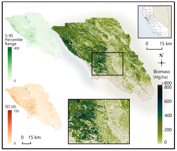
Figure 1. Estimated aboveground biomass (Mg/ha) for Sonoma County at 30 m spatial resolution with the 5th to 95th percentile range and the standard deviation (SD) of per-pixel biomass estimates shown in the top left and bottom left, respectively.
Citation
Duncanson, L., R.O. Dubayah, J. Armston, M. Liang, A. Arthur, and D. Minor. 2020. CMS: LiDAR Biomass Improved for High Biomass Forests, Sonoma County, CA, USA, 2013. ORNL DAAC, Oak Ridge, Tennessee, USA. https://doi.org/10.3334/ORNLDAAC/1764
Table of Contents
- Dataset Overview
- Data Characteristics
- Application and Derivation
- Quality Assessment
- Data Acquisition, Materials, and Methods
- Data Access
- References
Dataset Overview
This dataset provides estimates of aboveground woody biomass and uncertainty at 30 m spatial resolution for Sonoma County, California, USA, for the nominal year 2013. Biomass estimates, provided in megagrams of biomass per hectare (Mg/ha), were generated using a combination of airborne LiDAR data and field plot measurements. The relationship between field-estimated and airborne LiDAR-estimated aboveground biomass density is represented as a parametric model that predicts biomass as a function of canopy cover and 50th percentile and 90th percentile LiDAR heights at a 30 m resolution. To estimate uncertainty, the biomass model was re-fit 1,000 times through a sampling of the variance-covariance matrix of the fitted parametric model. This produced 1,000 estimates of biomass per pixel. The 5th and 95th percentiles and the standard deviation of the pixel biomass estimates were also calculated.
This dataset provides an updated aboveground woody biomass density map that builds upon the previously archived dataset Dubayah et al. (2017) (https://doi.org/10.3334/ORNLDAAC/1523). Differences between the two products are described.
Project: Carbon Monitoring System
The NASA Carbon Monitoring System (CMS) is designed to make significant contributions in characterizing, quantifying, understanding, and predicting the evolution of global carbon sources and sinks through improved monitoring of carbon stocks and fluxes. The System will use the full range of NASA satellite observations and modeling/analysis capabilities to establish the accuracy, quantitative uncertainties, and utility of products for supporting national and international policy, regulatory, and management activities. CMS will maintain a global emphasis while providing finer scale regional information, utilizing space-based and surface-based data and will rapidly initiate generation and distribution of products both for user evaluation and to inform near-term policy development and planning.
Related Datasets
Cook, B., A. Swatantran, L. Duncanson, A. Armstrong, N. Pinto, R. Nelson. 2014. CMS: LiDAR-derived Estimates of Aboveground Biomass at Four Forested Sites, USA. ORNL DAAC, Oak Ridge, Tennessee, USA. https://doi.org/10.3334/ORNLDAAC/1257
Dubayah, R.O., A. Swatantran, W. Huang, L. Duncanson, K. Johnson, H. Tang, J.O. Dunne, and G.C. Hurtt. 2016. CMS: LiDAR-derived Aboveground Biomass, Canopy Height and Cover for Maryland, 2011. ORNL DAAC, Oak Ridge, Tennessee, USA. https://doi.org/10.3334/ORNLDAAC/1320
Dubayah, R.O., A. Swatantran, W. Huang, L. Duncanson, H. Tang, K. Johnson, J.O. Dunne, and G.C. Hurtt. 2017. CMS: LiDAR-derived Biomass, Canopy Height and Cover, Sonoma County, California, 2013. ORNL DAAC, Oak Ridge, Tennessee, USA. https://doi.org/10.3334/ORNLDAAC/1523
- This previously archived dataset used the same LiDAR data and many of the same field plot data as the current, but a different modeling approach to derive biomass for Sonoma County. Differences from the new dataset are described below. This dataset will remain available because users may find strengths or weaknesses in either approach and may choose a product to meet their needs.
Acknowledgments
This research was funded by NASA Carbon Monitoring System grant 15-CMS15-0055.
Data Characteristics
Spatial Coverage: Sonoma County, California, USA
Spatial Resolution: 30-meter grid cells
Temporal Coverage: The dataset has no explicit temporal component. Data are nominally for the year 2013.
Temporal Resolution: One-time measurements
Study Area Latitudes and longitudes are provided in decimal degrees.
| Site | Westernmost Longitude | Easternmost Longitude | Northernmost Latitude | Southernmost Latitude |
|---|---|---|---|---|
| Sonoma County, California | -123.542 | -122.339 | 38.86417 | 38.10167 |
Data File Information
There are four data files in GeoTIFF (*.tif) provided with this dataset.
Table 1. File names and descriptions.
| Filename | Description |
|---|---|
| sonoma_biomass_pred.tif | Predicted woody aboveground biomass in megagrams per hectare for Sonoma County at 30 m spatial resolution. |
| sonoma_biomass_5pctl.tif | 5th percentile of estimated biomass per pixel in megagrams per hectare. Derived by re-fitting the biomass model 1,000 times through a sampling of the variance-covariance matrix of the fitted parametric model and calculating the 5th percentile for each pixel. |
| sonoma_biomass_95pctl.tif | 95th percentile of estimated biomass per pixel in megagrams per hectare. Derived by re-fitting the biomass model 1,000 times through a sampling of the variance-covariance matrix of the fitted parametric model and calculating the 95th percentile for each pixel. |
| sonoma_biomass_stddev.tif | The standard deviation of estimated biomass per pixel in megagrams per hectare. Derived by re-fitting the biomass model 1,000 times through a sampling of the variance-covariance matrix of the fitted parametric model and calculating the standard deviation for each pixel. |
Data File Details
All files have the same coordinate reference system "NAD83 / UTM zone 10N", EPSG: 26910, and the missing data value is -3.40E+38.
Application and Derivation
These data represent a reference biomass map for spaceborne biomass product evaluation. For this particular project, the reference map was for assessment and inter-comparison of simulated GEDI, ICESat-2, and NISAR (Duncanson et al., 2020), but this product can serve as a reference for any spaceborne biomass product that is temporally coincident with the 2013 LiDAR acquisition. Note that since 2013 significant fire activity has occurred, and thus caution is recommended when using this product for comparison to circa 2020 biomass products (e.g., GEDI and/or ICESat-2).
Quality Assessment
The current dataset is an updated biomass product based upon a previously archived dataset by Dubayah et al. (2017). This section briefly describes the differences between the old and new biomass estimates. Text and figures courtesy of the authors.
Note that the Dubayah et al. (2017) dataset will remain available because users may find strengths or weaknesses in either approach and may choose a product to meet their needs.
Old and New Biomass Maps Comparison
Both data products started with the same wall-to-wall LiDAR airborne data collected over Sonoma County in the fall of 2013 using Leica ALS50 and ALS70 instruments giving coverage over the whole county at 14 points m-2 (Dubayah et al., 2013).
Dubayah et al. (2017) reported a 30 m biomass map for all of Sonoma County (Dubayah et al., 2013) derived using a random forest model and calibrated with 166 field plots collected at a random sample of locations stratified by land cover type (Duncanson et al., 2017; Huang et al., 2017). Later analyses determined there was an underestimation of biomass in tall, high biomass forests across the County. The reasons for these underestimates were two-fold; first, the stratified random sample of the field biomass estimates did not capture the range and variability in some of Sonoma's tallest forests, and second, the random forest algorithm employed constrained estimates to the highest biomass field plot (517 Mg/ha).
In the current dataset, a new 30 m biomass map is provided (Fig. 1) that was generated using 30 additional plots sampled in high biomass redwood forests across the county and used a parametric modeling approach to estimate biomass (Fig. 2).
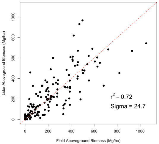
Figure 2. The model between field estimated and airborne LiDAR estimated Aboveground Biomass Density is a parametric model predicting biomass as a function of percent Canopy Cover, 50th percentile, and 90th percentile LiDAR heights at a 30 m resolution.
The differences between the old and new biomass estimates show that most of the changes in these maps are in the high biomass, tall forests, where the new map provides larger estimates (Fig. 3, Fig. 4). This was expected, both because of the inclusion of the new plots and the adoption of the parametric model that does not constrain the higher biomass estimates.
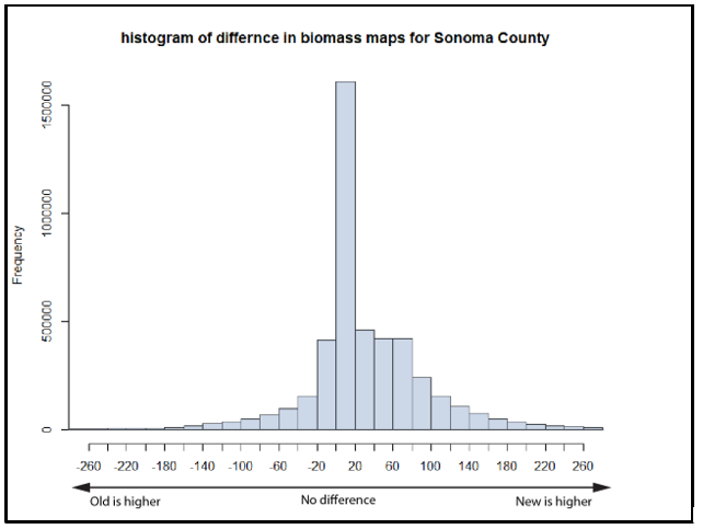
Figure 3. A histogram showing the differences between the new and old biomass map.
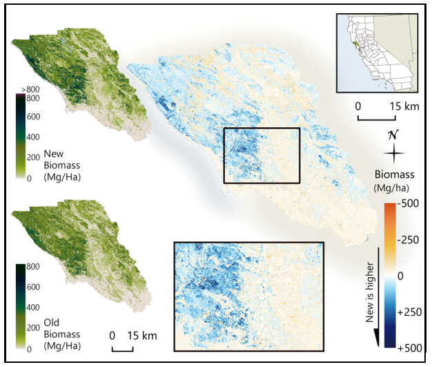
Figure 4. The difference between the previous Dubayah et al. (2017) random forest-based biomass map and this updated map is presented, with areas in blue representing where the new map provides higher estimates of biomass and orange/red showing where the new map provides lower estimates of biomass.
New Biomass Map Uncertainty Estimates
To estimate uncertainty, the biomass model was re-fit 1,000 times through a sampling of the variance-covariance matrix of the fitted parametric model. This produced 1,000 estimates of biomass per pixel. The 5th and 95th percentile, as well as the standard deviation of these pixel estimates, were calculated. Note that error was not propagated from field estimations (i.e., neither measurement error nor allometric error).
Data Acquisition, Materials, and Methods
This dataset provides an updated airborne LiDAR aboveground woody biomass density map at a 30 m resolution building upon the previously archive dataset Dubayah et al. (2017) (https://doi.org/10.3334/ORNLDAAC/1523).
The previous map underestimated biomass in tall, high biomass forests across the County. See the Quality Assessment section for a discussion of underestimations and the differences between the two map products.
Current Dataset Processing
The LiDAR data used are the same as used in Dubayah et al. (2017). Field plot data included the 166 field plots from Dubayah et al. (2017) and 30 new field reference plots that were randomly sampled in tall (>30 m) forests across the County.
The relationship between field estimated and airborne LiDAR estimated aboveground biomass density is a parametric model that predicts biomass as a function of percent Canopy Cover (Dubayah et al., 2017), and 50th percentile, and 90th percentile LiDAR heights at a 30 m resolution (Fig. 2).
To estimate uncertainty, the biomass model was re-fit 1,000 times through a sampling of the variance-covariance matrix of the fitted parametric model. This produced 1,000 estimates of biomass per pixel. The 5th and 95th percentile, as well as the standard deviation of these pixel estimates, were calculated. Note that error was not propagated from field estimations (neither measurement error nor allometric error).
A comparison between the revised and original maps shows the largest differences occur in the tallest forests, where the new map produces higher estimates than the original map.
Methods Background Information
Most of the information provided here is from Dubayah et al. 2017.
Field Plots
The 166 field sample plots were located and selected through a stratified sampling of land cover strata defined by the Classification Assessment with LANDSAT of Visible Ecological Groupings (CALVEG) land cover product (evergreen, deciduous, shrub, mixed and non-forest) and LiDAR canopy heights (low: 0 - 5 m, medium: 5 - 25 m and high: > 25 m). Tree measurements of diameter at breast height were recorded in each plot. Allometric estimates of AGB (Mg ha-1) were calculated for each tree using equations from FIA’s Component Ratio Method (Heath et al, 2008; Woodall et al., 2011) and appropriate blow-up factors were applied to estimate biomass density for the variable radius plots.
The 30 new field reference plots that were randomly sampled in tall (>30 m) forests across the County. Tree measurements and allometric biomass estimates were as noted above. All field data will be provided in a forthcoming dataset.
LiDAR Data
LiDAR data (~8 points/ sq.m.) were acquired over Sonoma County by Watershed Sciences Inc (WSI) in September–November of 2013 covering ~440,000 ha (44 flights). Airborne discrete return LiDAR instrument - Leica ALS70 sensor was mounted on a Cessna Grand Caravan. These data are available from several public sources. The LiDAR data were processed and classified to generate bare earth DEMs and Canopy Height Models for aboveground biomass estimation.
Tree Canopy Height and Cover
The tree canopy cover map was created using an object-based, data-fusion approach (LiDAR and high-resolution National Agriculture Imagery Program (NAIP) images), and then aggregated to 30-m by averaging. The canopy height map was generated using LiDAR-derived normalized digital surface model (ndsm) and tree cover map and then aggregated to 30-m by maximum (Huang et al., 2017).
Data Access
These data are available through the Oak Ridge National Laboratory (ORNL) Distributed Active Archive Center (DAAC).
CMS: LiDAR Biomass Improved for High Biomass Forests, Sonoma County, CA, USA, 2013
Contact for Data Center Access Information:
- E-mail: uso@daac.ornl.gov
- Telephone: +1 (865) 241-3952
References
Dubayah, R.O., A. Swatantran, W. Huang, L. Duncanson, K. Johnson, H. Tang, J.O. Dunne, and G.C. Hurtt. 2016. CMS: LiDAR-derived Aboveground Biomass, Canopy Height and Cover for Maryland, 2011. ORNL DAAC, Oak Ridge, Tennessee, USA. https://doi.org/10.3334/ORNLDAAC/1320
Dubayah, R.O., A. Swatantran, W. Huang, L. Duncanson, H. Tang, K. Johnson, J.O. Dunne, and G.C. Hurtt. 2017. CMS: LiDAR-derived Biomass, Canopy Height and Cover, Sonoma County, California, 2013. ORNL DAAC, Oak Ridge, Tennessee, USA. https://doi.org/10.3334/ORNLDAAC/1523
Duncanson, L., W. Huang, K. Johnson, A. Swatantran, R.E. McRoberts, and R. Dubayah. 2017. Implications of allometric model selection for county-level biomass mapping. Carbon Balance Manag. 12. https://doi.org/10.1186/s13021-017-0086-9
Duncanson, L., A. Neuenschwander, S. Hancock, N. Thomas, T. Fatoyinbo, M. Simard, C.A. Silva, J. Armston, S.B. Luthcke, M. Hofton, J.R. Kellner, and R. Dubayah. 2020. Biomass estimation from simulated GEDI, ICESat-2 and NISAR across environmental gradients in Sonoma County, California. Remote Sensing of Environment, 242: 111779. https://doi.org/10.1016/j.rse.2020.111779
Heath, L.S., M. Hansen, J.E. Smith, P.D. Miles, and B.W. Smith. 2008. Investigation into calculating tree biomass and carbon in the FIADB using a biomass expansion factor approach. In: McWilliams, Will; Moisen, Gretchen; Czaplewski, Ray, comps. Forest Inventory and Analysis (FIA) Symposium 2008; October 21-23, 2008; Park City, UT. Proc. RMRS-P-56CD. Fort Collins, CO: U.S. Department of Agriculture, Forest Service, Rocky Mountain Research Station. 26 p. https://www.fs.usda.gov/treesearch/pubs/33351
Huang, W., A. Swatantran, L. Duncanson, K. Johnson, D. Watkinson, K. Dolan, J. O’Neil-Dunne, G. Hurtt, and R. Dubayah. 2017. County-scale biomass map comparison: A case study for Sonoma, California. Carbon Management 8, 417–434. https://doi.org/10.1080/17583004.2017.1396840
Huang, W., A. Swatantran, K. Johnson, L. Duncanson, H. Tang, J. O'Neil Dunne, G. Hurtt, G., and R. Dubayah. 2015. Local Discrepancies in Continental Scale Biomass Maps: A Case Study over Forested and Non-Forested Landscapes in Maryland, USA. Carbon Balance and Management, 10. https://doi.org/10.1186/s13021-015-0030-9
Woodall, C., L.S. Heath, G.M. Domke, and M.C. Nichols. 2010. Methods and Equations for Estimating Aboveground Volume, Biomass, and Carbon for Trees in the US Forest Inventory. Gen. Tech. Rep. NRS-88. Newtown Square, PA: U.S. Department of Agriculture, Forest Service, Northern Research Station. 30 p. https://www.nrs.fs.fed.us/pubs/39555