Documentation Revision Date: 2021-04-01
Dataset Version: 1
Summary
GCReW, at the Smithsonian Environmental Research Center in Edgewater, MD, USA, is one of the most studied tidal wetlands in the world and is the source of many impactful insights on relationships among plant traits, microbial activity, and soil biogeochemical responses to global change factor interactions.
The DEMs are provided in four GeoTIFF (.tif) files, one for each DEM, and the model performance metrics are provided in one comma-separated (.csv) file.
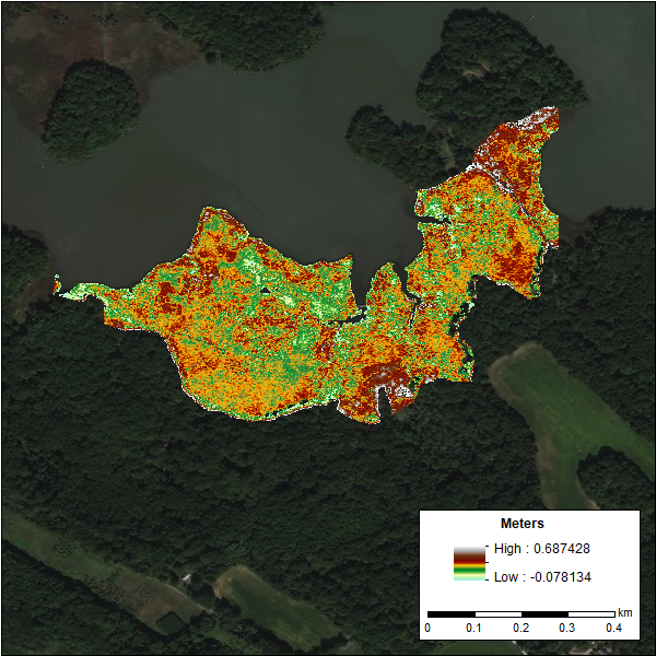
Figure 1. DEM of the Global Change Research Wetland (GCReW) site generated using the LiDAR Elevation Correction with NDVI (LEAN) method with existing LiDAR data and bias-corrected the LEAN algorithm. Source: GCReW_Elevation_2016_LEAN.tif
Citation
Holmquist, J.R., J. Riera, J.P. Megonigal, L. Schile-beers, K.J. Buffington, and D.E. Weller. 2021. Digital Elevation Models for the Global Change Research Wetland, Maryland, USA, 2016. ORNL DAAC, Oak Ridge, Tennessee, USA. https://doi.org/10.3334/ORNLDAAC/1793
Table of Contents
- Dataset Overview
- Data Characteristics
- Application and Derivation
- Quality Assessment
- Data Acquisition, Materials, and Methods
- Data Access
- References
Dataset Overview
This dataset contains four alternative digital elevation models (DEMs) at 1 m resolution and model performance statistical metrics for the Global Change Research Wetland (GCReW) site on the Rhode River, a tributary of the Chesapeake Bay in Maryland, USA, for the year 2016. Three DEMs were created by using different strategies for correcting positive biases in Light Detection and Ranging (LiDAR)-based DEMs that are common in tidal wetlands. These included (1) applying a single average offset based on a literature review, (2) using the LiDAR Elevation Correction with NDVI (LEAN)-method, and (3) applying plant community-specific offsets using a local vegetation cover map. Existing LiDAR data at 1 m resolution collected in 2011 was the basis for these DEMs. The fourth DEM was created by using Empirical Bayesian Kriging to extrapolate between measured ground points. The elevation is provided in meters relative to the North American Vertical Datum of 1988 (NAVD 88). To calibrate the four approaches, the elevation of the entire marsh complex was surveyed at 20 m x 20 m resolution to document the distribution of elevation relative to tidal datums from a single year. Two Trimble R8 real-time kinematic (RTK) GPS receivers were used to survey 525 points over the complex from July 26, 2016, to August 15, 2016. Relative plant cover was also documented. Tidal datums were calculated from the nearby Annapolis, MD tidal gauge located 13 km from GCReW.
GCReW, at the Smithsonian Environmental Research Center in Edgewater, MD, USA, is one of the most studied tidal wetlands in the world and is the source of many impactful insights on relationships among plant traits, microbial activity, and soil biogeochemical responses to global change factor interactions.
Project: Carbon Monitoring System
The NASA Carbon Monitoring System (CMS) is designed to make significant contributions in characterizing, quantifying, understanding, and predicting the evolution of global carbon sources and sinks through improved monitoring of carbon stocks and fluxes. The System will use the full range of NASA satellite observations and modeling/analysis capabilities to establish the accuracy, quantitative uncertainties, and utility of products for supporting national and international policy, regulatory, and management activities. CMS will maintain a global emphasis while providing finer scale regional information, utilizing space-based and surface-based data and will rapidly initiate generation and distribution of products both for user evaluation and to inform near-term policy development and planning.
Related Publications
Holmquist, J.R., L. Schile-Beers, K. Buffington, M. Lu, T.J. Mozdzer, J. Riera, D.E. Weller, M. Williams, and J.P. Megonigal. 2020. Scalability and Performance Tradeoffs in Quantifying Relationships between Elevation and Tidal Wetland Plant Communities. In preparation.
Acknowledgments
This work was funded by NASA’s CMS program with grant number NNH14AY67I.
Data Characteristics
Spatial Coverage: The Rhode River wetland, a tributary of the Chesapeake Bay, Maryland, USA
Spatial Resolution: 1 meter
Temporal Coverage: 2016-06-22 to 2016-08-15
Temporal Resolution: One-time measurements in the year 2016
Site Boundaries: Latitude and longitude are given in decimal degrees.
| Site (Region) | Westernmost Longitude | Easternmost Longitude | Northernmost Latitude | Southernmost Latitude |
|---|---|---|---|---|
| Rhode River, MD | -76.5429 | -76.5521 | 38.8789 | 38.87172 |
Data File Information
There are four data files in GeoTIFF (.tif) format, and one file in comma-separated (.csv) format with this dataset.
Table 1. File names and descriptions.
| File Names | Description |
|---|---|
| GCReW_Elevation_2016_SingleAdjustment.tif | DEM created using existing LiDAR dataset and bias-corrected using an assumption of an average offset from a literature review |
| GCReW_Elevation_2016_LEAN.tif | DEM created using existing LiDAR dataset and bias-corrected the LEAN algorithm |
| GCReW_Elevation_2016_EBK.tif | DEM created using empirical bayesian kriging |
| GCReW_Elevation_2016_VegZoneCorrection.tif | DEM created using existing LiDAR dataset and bias-corrected using average offsets for different vegetation community zones |
| DEM_performance_statistics.csv | This file provides various performance metrics of the four methods |
Data File Details
- Elevation was measured in meters relative to NAVD 88
- The projection is "WGS 84", EPSG:4326
- Map units: degree
- Map resolution: ~1 m (~ 0.00001 degrees)
- No data value: -9999
Table 2. Variables in the data file DEM_performance_statistics.csv.
| Column | Units | Description |
|---|---|---|
| DEM_analysis_code | categories |
Code indicating the analysis used to generate the DEM:
|
| bias | meters | Mean of the residuals |
| unbiasedRmse | meters | Unbiased Root Mean Square Error, the standard deviation of the residuals after taking into account bias. Note that these values are artificially signed so that models that overestimate variance are positive and those that underestimate variance are negative. |
| totalRmse | meters | Total Root Mean Square Error, the sum of squares of Bias and Unbiased Root Mean Square Error. |
| standardizedBias | dimensionless | Mean of the residuals normalized by the standard deviation of the reference dataset. |
| standardizedUnbiasedRmse | dimensionless | Unbiased Root Mean Square Error, the standard deviation of the residuals after taking into account bias, and normalized by the standard deviation of the reference dataset. Note that these values are artificially signed so that models that overestimate variance are positive and those that underestimate variance are negative. |
| standardizedTotalRmse | dimensionless | Total Root Mean Square Error, the sum of squares of Bias and Unbiased Root Mean Square Error, and normalized by the standard deviation of the reference dataset. Note that when the total standardized Root Mean Square Error is less than 1, it means the model performs better than simply applying the average from the calibration dataset. |
Application and Derivation
The GCReW is one of the most studied sites in the world, and accurate and precise geospatial information on its elevation is needed to apply dynamic numerical models of elevation change and carbon sequestration driven by projected sea-level rise.
Quality Assessment
An independently collected and held-out RTK-GPS survey dataset was used to intercompare the four DEM strategies based on bias, unbiased-root mean square error, total root mean square error, and whether or not the DEM over- or under-estimated variance in the elevation surface. Refer to the data file DEM_performance_statistics.csv for the DEM performance statistics.
Data Acquisition, Materials, and Methods
Following is a brief synopsis of methods provided in Holmquist et al. (2020).
Site Description
GCReW at the Smithsonian Environmental Research Center in Edgewater, MD, USA, is one of the most studied tidal wetlands in the world and is the source of many impactful insights on relationships among plant traits, microbial activity, and soil biogeochemical responses to global change factor interactions. GCReW occupies about half of a larger 22 ha marsh complex known locally as Kirkpatrick Marsh. Despite the intensive, long-term experiments at GCReW, no previous study has documented the natural history of important vegetation-elevation relationships and tidal datums at the site.
Elevation, tidal datums, plant cover surveys, and kriging were used to generate four unbiased wetland DEMs of the entire marsh complex at 20 m x 20 m resolution and to document the distribution of elevation relative to tidal datums from a single year.
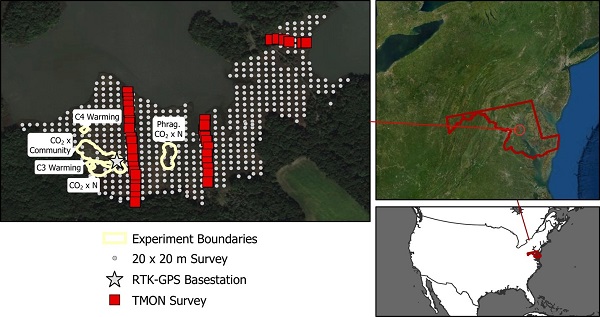
Figure 2. Marsh extent and the boundaries of existing experiments at the Global Change Research Wetland, as well as the 20 m x 20 m elevation and vegetation survey grid and the Tennenbaum Marine Observatory Network (TMON) plots. Inserts show the site in relation to the state of Maryland and the United States. Source: Holmquist et al., (2020)
Tidal Datum Transformations
Elevation data were summarized relative to tidal datums that were calculated from the nearby Annapolis MD tidal gauge located 13 km from GCReW. A suite of tidal datums (NOAA 2020a) was calculated for 2016 from complete, verified, 6-minute tide gauge data. Tides were predicted at the same 6-minute resolution as the data using a nearest neighbor analysis to isolate high and low tides, then differentiated higher high tides from lower high tides, and lower low tides from higher low tides (NOAA 2020b).
Marsh Elevation and Plant Community Surveys
Trimble R8 real-time kinematic (RTK) GPS receivers were used for two separate elevation surveys; one of the vegetation plots measured as part of the Smithsonian’s Tennenbaum Marine Observatory Network (TMON), and the other a 20 m x 20 m grid over most of Kirkpatrick Marsh.
For the 20 m x 20 m grid survey, an outline was created of the contiguous section of the wetland using high-resolution Google Earth Imagery and polygons delineated by the National Wetlands Inventory (NWI; USFWS 2014). The outlines of major features were digitized on the marsh such as boardwalks and experimental chambers. At the time of this survey, the warming experiments and new boardwalks had not been captured in the high-resolution Google Earth Imagery, so the boundaries were surveyed of these experiments and boardwalks. A 20 m x 20 m grid was created and converted to center points, then the points were subsetted that intersected the marsh, and those within a 5 m buffer of site infrastructure or the TMON plots were omitted.
The entire 525-point grid was surveyed between July 26, 2016, and August 15, 2016. If a planned elevation point did not intersect the marsh as mapped because of trees, creeks, or marsh edges, the point was moved to the nearest access. In some places, the edges of the marsh were opportunistically surveyed if they were either near a sampling point or if the edge of the marsh was not visible in the imagery used to plan the survey. RTK-GPS data were post-processed (Holmquist et al., 2020).
In conjunction with the grid-based elevation survey, plant community presence, absence, and relative abundance were recorded.
Generation of DEMs
Methods to generate four unbiased DEMs included: (1) applying a single average offset from a literature review of coastal wetland studies that performed bias corrections to LiDAR-based DEMs, (2) using the LEAN algorithm to correct a LiDAR-based DEM, (3) applying vegetation community-specific corrections to correct a LiDAR-based DEM, and (4) using spatial interpolation among points instead of a LiDAR-based DEM. For the three LiDAR-based techniques, Lidar-based DEMs were used from an Anne Arundel County LiDAR-based DEM created from imagery flown in 2011, and a 1 m resolution DEM produced by the Sanborn Map Company for county-wide FEMA flood map modernization. The LiDAR flight and the RTK-GPS survey were four years apart, but it was assumed that any accretion or subsidence over that time would be within the nominal error of the RTK-GPS. The four methods are further described below.
(1) Applying a single average offset from a literature review of coastal wetland studies that performed bias corrections to LiDAR-based DEMs
This DEM was created as in Holmquist et al. (2018) from previously collected data for wetland surfaces based on a weighted average of results from multiple US-based studies. Wetland vegetation and soil introduce system-specific bias and random error not captured by the nominal accuracy reporting. The DEM was corrected for a mean error of 0.172 m and subtracted from the LiDAR-based DEM elevation. This simple calculation required no new data collection, and it provided a base for evaluating more complex correction methods.
(2) Using the LEAN algorithm to correct a LiDAR-based DEM
This DEM was created using the Lidar Elevation Adjustment with NDVI (LEAN) method used in Buffington et al. (2016). LEAN uses ground measurements of elevation, typically from RTK-GPS, to calculate the vertical bias in LiDAR datasets. Initial LiDAR elevation and the Normalized Difference Vegetation Index (NDVI = ([NIR-Red]/[NIR+Red]; Red wavelength = 608-662 nm, NIR wavelengths=833-887 nm) from National Agriculture Imagery Program (NAIP; NAIP 2019) were used in a multivariate linear regression model to estimate the bias. NDVI is assumed to be a metric of vegetation height and density. All RTK-GPS marsh elevation points were used from the 20 m x 20 m grid survey to calibrate LEAN. The 4-band NAIP used to calculate NDVI was acquired on July 24, 2015. To estimate model skill, a 10-fold cross-validation procedure was used in which the model was iteratively fit with 90% of the elevation data and tested against the 10% hold out.
(3) Applying vegetation community-specific corrections to correct a LiDAR-based DEM
A digitized map of GCReW vegetation zones was used to test applying cover-based elevation bias corrections. The map used consisted of six major vegetation cover types: an Iva frutescens-dominated community, an I. frutescens, and Phragmites australis-mixed community, a Schenoplectus americanus and Spartina patens mixed community, a P. australis-dominated community, and an S. americanus-dominated community, and an S. patens-dominated community. Community boundaries were delineated by trained personnel using high resolution 2010 summer imagery in Google Earth. Polygons were assigned one of six vegetation types using a supervised classifier in ArcGIS, trained using 26 ground-based reference points that were collected in 2014. This map was created for a separate, unpublished project. The vegetation communities in 2010 were compared to those delineated from an image taken in 1973 (NASA contractor report "Collection and analysis of remotely sensed data from the Rhode River Estuary Watershed" 1973, NASA CR-62094).
Analysis of variance (ANOVA) was used to test if there were significant differences between measured and mapped LiDAR-based elevation from the 20 m x 20 m grid survey, using the mapped vegetation community in the 2010 map as an independent variable and LiDAR offset as the dependent variable. If the relationship was significant, then a new DEM could be created by subtracting those vegetation offsets from the mapped surface (Holmquist et al., 2020).
(4) Using spatial interpolation (Kriging) among points instead of a LiDAR-based DEM
Empirical Bayesian Kriging was applied to all marsh surface data from the 20 m x 20 m grid survey. The median prediction and standard error of the krigged surface using a power semivariogram, and a 100 maximum point standard circular neighborhood with a radius of 272 m were both mapped (Holmquist et al., 2020).
Elevation Mapping Method Comparison
The four techniques were compared by validating each of the four maps with the TMON elevation plot measurements, which were independent of all vegetation height correction strategies. The mean error, a metric of bias, and unbiased root mean square error (RMSE’), which is a metric of precision were calculated. The metrics were normalized to the standard deviation of the reference dataset. The total RMSE, the sum of squares of ME and RMSE were also calculated.
Data Access
These data are available through the Oak Ridge National Laboratory (ORNL) Distributed Active Archive Center (DAAC).
Digital Elevation Models for the Global Change Research Wetland, Maryland, USA, 2016
Contact for Data Center Access Information:
- E-mail: uso@daac.ornl.gov
- Telephone: +1 (865) 241-3952
References
Buffington, K.J., B.D. Dugger, K.M. Thorne, and J.Y. Takekawa. 2016. Statistical correction of lidar-derived digital elevation models with multispectral airborne imagery in tidal marshes. Remote Sens Environ 186:616–625. https://doi.org/10.1016/j.rse.2016.09.020
Holmquist, J.R., L. Schile-Beers, K. Buffington, M. Lu, T.J. Mozdzer, J. Riera, D.E. Weller, M. Williams, and J.P. Megonigal. 2020. Scalability and Performance Tradeoffs in Quantifying Relationships between Elevation and Tidal Wetland Plant Communities. In preparation.
Holmquist, J.R., L. Windham-Myers, B. Bernal, K.B. Byrd, S. Crooks , M.E. Gonneea, N. Herold, S.H. Knox, K.D. Kroeger, J. McCombs, J. Patrick Megonigal, M. Lu, J.T. Morris, A.E. Sutton-Grier, T.G. Troxler, and D.E. Weller. 2018. Uncertainty in United States coastal wetland greenhouse gas inventorying. Environ Res Lett 13:115005. https://doi.org/10.1088/1748-9326/aae157
USFWS. 2014. National Wetlands Inventory website. U.S. Department of the Interior, Fish and Wildlife Service, Washington, D.C. http://www.fws.gov/wetlands/
NOAA. 2020a. National Oceanic and Atmospheric Administration Tides and Currents: Datums. https://tidesandcurrents.noaa.gov/datums.html?datum=MLLW&units=1&epoch=0&id=8575512&name=Annapolis&state=MD
NOAA. 2020b. National Oceanic and Atmospheric Administration Tides and Currents: Sea Level Trends https://tidesandcurrents.noaa.gov/sltrends/sltrends_station.shtml?id=8575512
NAIP. 2019. National Agriculture Imagery Program https://datagateway.nrcs.usda.gov/GDGHome_DirectDownLoad.aspx