Documentation Revision Date: 2025-09-15
Dataset Version: 2
Summary
In this 2nd edition of the data product, lidar-derived AGB maps were calibrated with Forest Inventory and Analysis (FIA) plot data. For each state (WA, OR, and ID-MT), a simple linear model was fit to regress FIA subplot estimates on the lidar landscape estimates at the FIA subplot locations (Table 1), then applied to the lidar landscape mean and standard deviation estimates of AGB within their respective states. Note that the AGB estimates are, for the most part, a single snapshot in time and that the forest conditions are not necessarily representative of the larger study area. The data are provided in GeoTIFF, shapefile, and Keyhole Markup Language formats.
Table 1. Simple linear regression coefficients used to calibrate AGB maps.
|
State |
Intercept |
Slope |
|
Washington |
-35.9416918612722 |
1.39232989981623 |
|
Oregon |
-12.3316457744595 |
1.29708601817535 |
|
Idaho/Montana |
-7.33080981257064 |
1.11332686381382 |
There are 354 files in this dataset: one biomass estimate and standard deviation file for each of the 176 lidar collections in GeoTIFF format, one shapefile in a compressed Zip archive, and one file in Keyhole Markup Language (KMZ) format.
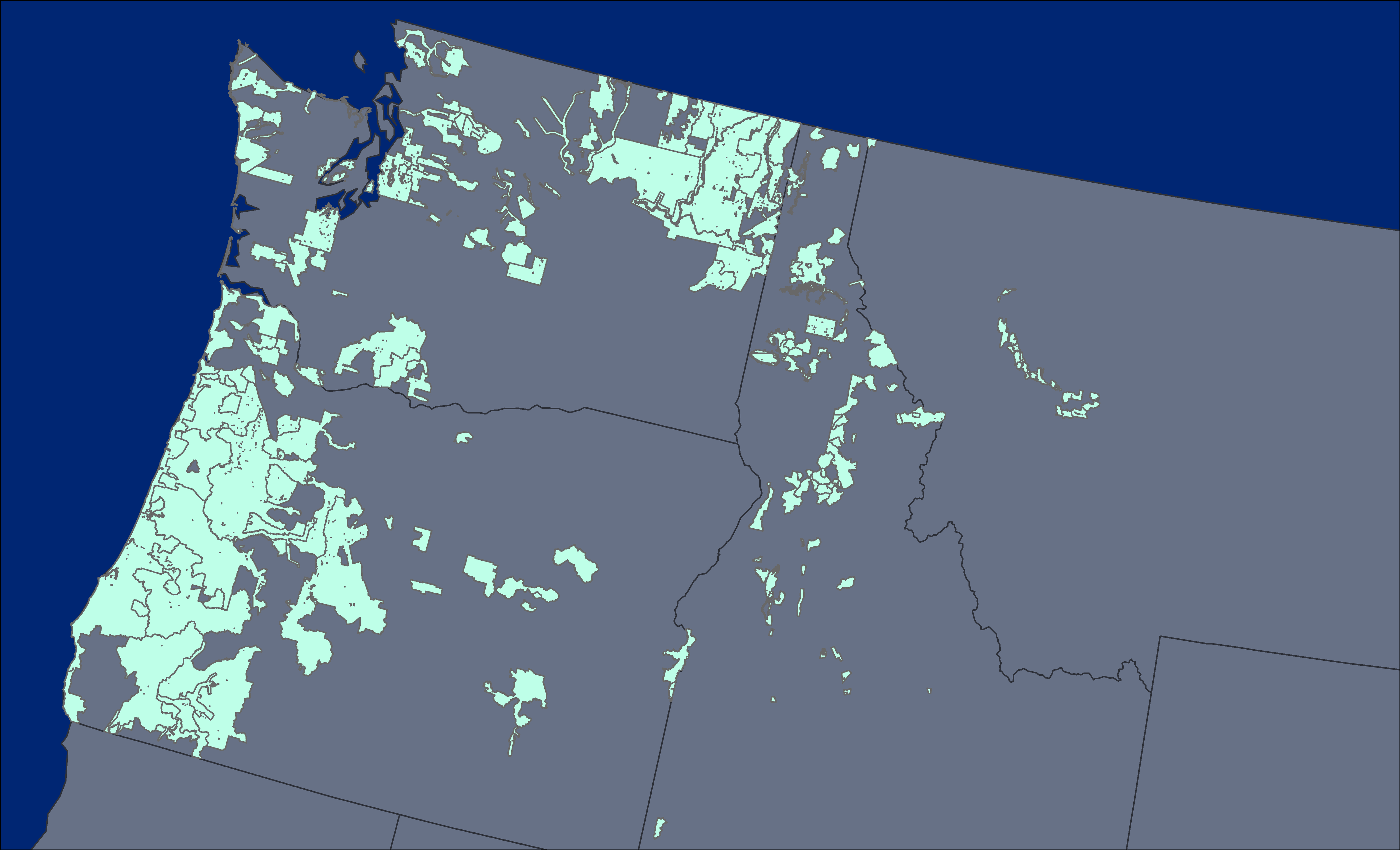
Figure 1. The locations of the 176 lidar collection areas (light green polygons) acquired between 2002 and 2016. Source: Forest_AGB_NW_LidarUnits.zip
Citation
Fekety, P.A., A.T. Hudak, and B.C. Bright. 2025. LiDAR-derived Forest Aboveground Biomass Maps, Northwestern USA, 2002-2016, V2. ORNL DAAC, Oak Ridge, Tennessee, USA. https://doi.org/10.3334/ORNLDAAC/2443
Table of Contents
- Dataset Overview
- Data Characteristics
- Application and Derivation
- Quality Assessment
- Data Acquisition, Materials, and Methods
- Data Access
- References
- Dataset Revisions
Dataset Overview
This dataset provides maps of aboveground forest biomass (AGB) of living trees and standing dead trees in Mg/ha across portions of northwestern United States, including Washington, Oregon, Idaho, and Montana, at a spatial resolution of 30 m. Forest inventory data were compiled from 29 stakeholders that had overlapping lidar imagery. The collection totaled 3,805 field plots with lidar imagery for 176 collections acquired between 2002 and 2016. Plot-level AGB estimates were calculated from tree measurements using the default allometric equations found in the Fire Fuels Extension (FFE) of the Forest Vegetation Simulator (FVS). The random forest algorithm was used to model AGB from lidar height and density metrics that were generated from the lidar returns within fixed-radius field plot footprints, gridded climate metrics obtained from the Climate-FVS Ready Data Server, and topographic estimates extracted from Shuttle Radar Topography Mission (SRTM) 1 Arc-Second Global elevation rasters. AGB was then mapped from the same lidar metrics gridded across the extent of the lidar collections at 30-m resolution. The standard deviation of estimated AGB of the terminal nodes from the random forest predictions was also mapped to show pixel-level model uncertainty. In this 2nd edition of the data product, lidar-derived AGB maps were calibrated with Forest Inventory and Analysis (FIA) plot data. For each state (WA, OR, and ID-MT), a simple linear model was fit to regress FIA subplot estimates on the lidar landscape estimates at the FIA subplot locations, then applied to the lidar landscape mean and standard deviation estimates of AGB within their respective states. Note that the AGB estimates are, for the most part, a single snapshot in time and that the forest conditions are not necessarily representative of the larger study area.
Project: Carbon Monitoring System
The NASA Carbon Monitoring System (CMS) program is designed to make significant contributions in characterizing, quantifying, understanding, and predicting the evolution of global carbon sources and sinks through improved monitoring of carbon stocks and fluxes. The System uses NASA satellite observations and modeling/analysis capabilities to establish the accuracy, quantitative uncertainties, and utility of products for supporting national and international policy, regulatory, and management activities. CMS data products are designed to inform near-term policy development and planning.
Related Publication
Hudak, A. T., P. A. Fekety, V. R. Kane, R. E. Kennedy, S. K. Filippelli, M. J. Falkowski, W. T. Tinkham, A. M. S. Smith, N. L. Crookston, G. M. Domke, M. V. Corrao, B. C. Bright, D. J. Churchill, P. J. Gould, R. J. McGaughey, J. T. Kane, and J. Dong. 2020. A carbon monitoring system for mapping regional, annual aboveground biomass across the northwestern USA. Environmental Research Letters 15:095003. https://doi.org/10.1088/1748-9326/ab93f9
Related Datasets
Fekety, P.A., and A.T. Hudak. 2019. Annual Aboveground Biomass Maps for Forests in the Northwestern USA, 2000-2016. ORNL DAAC, Oak Ridge, Tennessee, USA. https://doi.org/10.3334/ORNLDAAC/1719
Filippelli, S.K., M.J. Falkowski, A.T. Hudak, and P.A. Fekety. 2020. CMS: Pinyon-Juniper Forest Live Aboveground Biomass, Great Basin, USA, 2000-2016. ORNL DAAC, Oak Ridge, Tennessee, USA. https://doi.org/10.3334/ORNLDAAC/1755
Fekety, P.A., A.T. Hudak and B.C. Bright. 2020. Tree and stand attributes for "A carbon monitoring system for mapping regional, annual aboveground biomass across the northwestern USA". Fort Collins, CO: Forest Service Research Data Archive. https://doi.org/10.2737/RDS-2020-0026
Acknowledgments
This work was supported by the NASA Carbon Monitoring System (NNH15AZ06I).
Data Characteristics
Spatial Coverage: Northwestern United States: Washington, Oregon, Idaho, and part of western Montana
Spatial Resolution: 30 m
Temporal Coverage: 2002 to 2016 (actual temporal coverage varies across Lidar units)
Temporal Resolution: one-time estimates
Study Area: Latitude and longitude are given in decimal degrees.
| Region | Westernmost Longitude | Easternmost Longitude | Northernmost Latitude | Southernmost Latitude |
|---|---|---|---|---|
| Northwestern United States | -127.0456 | -111.399 | 50.4046 | 40.950 |
Data File Information
There are 354 files in this dataset: one aboveground biomass (AGB) estimate and standard deviation file for each of the 176 lidar collections in GeoTIFF format (*.tif), one shapefile in a compressed Zip archive (*.zip), and one file in Keyhole Markup Language (KMZ, *.kmz) format (Table 1).
The GeoTIFF files hold estimates of forest AGB for 176 lidar collections across the northwestern US. There are two GeoTIFFs per collection. The file naming convention is <LidarUnit>.tif (mean AGB estimates) and <LidarUnit>_StdDev.tif (standard deviations of the estimates).
<LidarUnit> in the GeoTIFF filename corresponds to the "LidarUnit" attribute of the shapefile in LidarUnits.zip.
The <LidarUnit> text varies according to the original lidar data stakeholder or host. Generally, the text begins with a name to describe the geographic location followed by the calendar year the lidar unit was captured. Some filenames include the date (YYYY-MM-DD) the files were processed.
Example GeoTIFF file names: Glacier_Peak_2010.tif, Glacier_Peak_2010_StdDev.tif,
GlacierPeak2015_2018-02-21.tif, GlacierPeak2015_2018-02-21_StdDev.tif, Glover2016.tif, Glover2016_StdDev.tif
GeoTIFF characteristics:
- Coordinate system: Conus Albers projection using NAD83 datum (EPSG:5070); units = meters
- Pixel values: forest aboveground biomass in megagrams per hectare
- Data type: Int16
- Nodata value: 65535
Table 1. File names and descriptions.
| File Name | Units | Description |
|---|---|---|
| <LidarUnit>.tif | Mg ha-1 | 176 files of forest aboveground forest biomass (AGB, living trees and standing dead trees) at 30-m resolution within the LidarUnit. |
| <LidarUnit>_StdDev.tif | Mg ha-1 | 176 files of the standard deviation of forest AGB of the terminal nodes from the random forests predictions. |
| Forest_AGB_NW_LidarUnits.zip | A shapefile in a Zip archive holding the polygons for the 176 LidarUnits. Shapefile attributes include:
|
|
| Forest_AGB_NW_LidarUnits.kmz | Compressed Keyhole Markup Language file to visualize the 176 LidarUnits in Google Earth. |
Application and Derivation
This dataset provides estimates of AGB from plot scale field and lidar measurements that match in space and time (Hudak et al., 2020).
Quality Assessment
Quality Assessment
Highly correlated explanatory variables (r ≥ 0.9) were removed and model selection was used to select a parsimonious model of AGB. Model fit was based on 500 trees and assessed through the pseudo-R2 statistic. The standard deviation of estimated AGB calculated across the 500 trees were mapped to show pixel-level model uncertainty. In this 2nd edition of the data product, lidar-derived AGB maps were calibrated with FIA plot data. For each state (WA, OR, and ID-MT), a simple linear model was fit to regress FIA subplot estimates on the lidar landscape estimates at the FIA subplot locations, then applied to the lidar landscape mean and standard deviation estimates of AGB within their respective states. See Hudak et al. (2020) for details.
Data Acquisition, Materials, and Methods
Forest inventory data collected by 29 stakeholders (federal, state, university, and private organizations) were compiled for a total of 3,805 field plots. The field plots were established within three years of an overlapping lidar collection and were not disturbed in the time between field and lidar data collections. At all field plots, a minimum of species, status (live or dead), and diameter at breast height (DBH) were recorded for all trees with a DBH greater than or equal to 12.7 cm, and tree heights were measured for a sample of the trees.
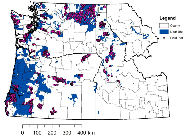
Figure 2. Study area with field plots and lidar collection areas. Source: Hudak et al. (2020).
Aboveground biomass (AGB) was calculated from tree measurements using the default equations found in the Fire and Fuels Extension to the Forest Vegetation Simulator (Rebain 2015). The aboveground portion of the live and standing dead trees were summed to a single, plot-level AGB value.
Local and regional databases were searched to identify discrete airborne lidar collections acquired between 2002 and 2016 and located in forested ecoregions of the study area. In total, 13,007,443 ha of lidar coverages were processed. Plot-level lidar metrics were calculated by clipping and height-normalizing the lidar point cloud.
Plot-level AGB estimates served as the response variable for the random forests (RF) machine-learning algorithm to model AGB across the extent of the lidar coverage. Predictor variables included the plot-level lidar metrics, gridded climate metrics (1961-1990 normals) obtained from the Climate-FVS Ready Data Server (Crookston, 2016), and plot-level topographic estimates, calculated as the area-weighted mean of the pixel values intersecting the plot footprint, were extracted from SRTM1 Arc-Second Global elevation rasters (USGS, 2018). The project-level tree measurements and the plot attributes that were used to train the landscape mapped AGB estimates can be found at https://doi.org/10.2737/RDS-2020-0026
AGB was then mapped from the same lidar metrics gridded across the extent of the lidar collections at 30-m resolution. The standard deviation of estimated AGB of the terminal nodes from the random forest predictions was also mapped to show pixel-level model uncertainty. In this 2nd edition of the data product, lidar-derived AGB maps were calibrated with FIA plot data. For each state (WA, OR, and ID-MT), a simple linear model was fit to regress FIA subplot estimates on the lidar landscape estimates at the FIA subplot locations, then applied to the lidar landscape mean and standard deviation estimates of AGB within their respective states. Note that the AGB estimates are, for the most part, a single snapshot in time and that the forest conditions are not necessarily representative of the larger study area.
See Hudak et al. (2020) for details.
Data Access
These data are available through the Oak Ridge National Laboratory (ORNL) Distributed Active Archive Center (DAAC).
LiDAR-derived Forest Aboveground Biomass Maps, Northwestern USA, 2002-2016, V2
Contact for Data Center Access Information:
- E-mail: uso@daac.ornl.gov
- Telephone: +1 (865) 241-3952
References
Crookston, N. 2016. Climate estimates and plant-climate relationships. Climate-FVS. http://charcoal.cnre.vt.edu/climate/customData/fvs_data.php
Fekety, P.A., and A.T. Hudak. 2019. Annual Aboveground Biomass Maps for Forests in the Northwestern USA, 2000-2016. ORNL DAAC, Oak Ridge, Tennessee, USA. https://doi.org/10.3334/ORNLDAAC/1719
Fekety, P.A., A.T. Hudak, and B.C. Bright. 2020. Tree and stand attributes for "A carbon monitoring system for mapping regional, annual aboveground biomass across the northwestern USA". Forest Service Research Data Archive; Fort Collins, Colorado. https://doi.org/10.2737/RDS-2020-0026
Filippelli, S.K., M.J. Falkowski, A.T. Hudak, and P.A. Fekety. 2020. CMS: Pinyon-Juniper Forest Live Aboveground Biomass, Great Basin, USA, 2000-2016. ORNL DAAC, Oak Ridge, Tennessee, USA. https://doi.org/10.3334/ORNLDAAC/1755
Hudak, A. T., P. A. Fekety, V. R. Kane, R. E. Kennedy, S. K. Filippelli, M. J. Falkowski, W. T. Tinkham, A. M. S. Smith, N. L. Crookston, G. M. Domke, M. V. Corrao, B. C. Bright, D. J. Churchill, P. J. Gould, R. J. McGaughey, J. T. Kane, and J. Dong. 2020. A carbon monitoring system for mapping regional, annual aboveground biomass across the northwestern USA. Environmental Research Letters 15:095003. https://doi.org/10.1088/1748-9326/ab93f9
Rebain, S.A. 2010. (revised March 23, 2015). The Fire and Fuels Extension to the Forest Vegetation Simulator: Updated Model Documentation. Internal Report. U.S. Department of Agriculture, Forest Service, Forest Management Service Center; Fort Collins, Colorado. https://www.fs.usda.gov/fmsc/ftp/fvs/docs/gtr/FFEguide.pdf
USGS (United States Geological Survey). 2018. USGS EROS Archive - Digital Elevation - Shuttle Radar Topography Mission (SRTM) 1 Arc-Second Global. https://dx.doi.org/10.5066/F7PR7TFT
Dataset Revisions
| Version | Release Date | Revision Notes |
|---|---|---|
| 2.0 | 2025-09-15 | Lidar-derived AGB maps were calibrated with FIA plot data. |
| 1.0 | 2020-06-30 | Original Version 1 release (https://doi.org/10.3334/ORNLDAAC/1766). |