Documentation Revision Date: 2022-12-02
Dataset Version: 1
Summary
There are 59,416 data files in GeoTIFF (*.tif) format included in this dataset that provide the percent of ground covered by a lifeform class. The file count is summarized by 59,416 files = (425 tiles x 35 years x 4 cover types) - 84 files removed owing to missing data, as there are 425 tiles that span the spatial extent of CONUS, each tile spans 35 years, and there are four cover types per year. Each file contains four bands.
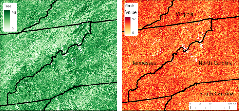
Figure 1. Percent cover of trees (left) and shrubs (right) in 2018 for the southern Appalachian mountains of Tennessee, Virginia, North Carolina, and South Carolina. Areas shown cover four tiles. Source: LPC_h024v011_SC_2018_V01.tif, LPC_h024v012_SC_2018_V01.tif, LPC_h025v011_SC_2018_V01.tif, LPC_h025v012_SC_2018_V01.tif, LPC_h024v011_TC_2018_V01.tif, LPC_h024v012_TC_2018_V01.tif, LPC_h025v011_TC_2018_V01.tif, LPC_h025v012_TC_2018_V01.tif.
Citation
Parra, A., and J.A. Greenberg. 2021. CMS: Vegetative Lifeform Cover from Landsat SR for CONUS, 1984-2018. ORNL DAAC, Oak Ridge, Tennessee, USA. https://doi.org/10.3334/ORNLDAAC/1809
Table of Contents
- Dataset Overview
- Data Characteristics
- Application and Derivation
- Quality Assessment
- Data Acquisition, Materials, and Methods
- Data Access
- References
Dataset Overview
This dataset contains estimates of percent cover of tree, shrub, herb, and other (non-vegetation) lifeform classes and uncertainties for the conterminous U.S. (CONUS). The estimates were derived using quantile regression forest models and indicate the percent of ground covered by a vertical projection of each lifeform class ranging from 0 to 100 percent. Model input data included Landsat surface reflectance (SR) data and 165 airborne LiDAR datasets covering eight of the eleven terrestrial biomes of the conterminous U.S. and Alaska, as defined by Olson et al. (2001). Eighty-six of the LiDAR acquisitions are part of the NASA Goddard's LiDAR, Hyperspectral, and Thermal Imager (G-LiHT) airborne imager data collection; the remaining 79 sites were acquired by the National Science Foundation's National Ecological Observatory Network Airborne Observation Platform (NEON AOP). Acquisitions were selected based on the availability of the SR data for each G-LiHT and NEON dataset. The data are annual estimates from 1984 to 2018 and were tiled (425 tiles) using the CONUS Landsat Analysis Ready Data (ARD) grid scheme.
Project: Carbon Monitoring System
The NASA Carbon Monitoring System (CMS) is designed to make significant contributions in characterizing, quantifying, understanding, and predicting the evolution of global carbon sources and sinks through improved monitoring of carbon stocks and fluxes. The System will use the full range of NASA satellite observations and modeling/analysis capabilities to establish the accuracy, quantitative uncertainties, and utility of products for supporting national and international policy, regulatory, and management activities. CMS will maintain a global emphasis while providing finer scale regional information, utilizing space-based and surface-based data, and will rapidly initiate generation and distribution of products both for user evaluation and to inform near-term policy development and planning.
Related Publication
A. Parra and J. A. Greenberg, "Estimation of Fractional Plant Lifeform Cover for the Conterminous United States Using Landsat Imagery and Airborne LiDAR," in IEEE Transactions on Geoscience and Remote Sensing, vol. 60, pp. 1-14, 2022, Art no. 4413614, doi: 10.1109/TGRS.2022.3199156
Acknowledgments
This research was funded under the NASA Carbon Monitoring System (grant NNX14AO80G).
Data Characteristics
Spatial Coverage: conterminous United States
Spatial Resolution: 30 m
Temporal Coverage: 1984-01-01 to 2018-01-01
Temporal Resolution: annual
Study Area: Latitude and longitude are given in decimal degrees.
| Sites | Westernmost Longitude | Easternmost Longitude | Northernmost Latitude | Southernmost Latitude |
|---|---|---|---|---|
| Conterminous U.S. | -126.7144194 | -65.06382101 | 50.66253889 | 23.26634323 |
Data File Information
There are 59,416 data files in GeoTIFF (*.tif) format included in this dataset that provide the percent of ground covered by a lifeform class. The file count is summarized by 59,416 files = (425 tiles x 35 years x 4 cover types) - 84 files removed owing to missing data, as there are 425 tiles that span the spatial extent of CONUS, each tile spans 35 years, and there are four cover types per year. Each file contains four bands (Table 2).
The files are named LPC_h###v###_XX_YYYY_V01.tif (e.g, LPC_h020v015_TC_1988_V01.tif), where
LPC = "Lifeform Percent Cover",
h###v### = tile designated by the CONUS Landsat ARD grid scheme: h### indicates the horizontal identifier of the tile and v### indicates the vertical identifier of the tile,
XX = lifeform cover class ("HC", "SC", "TC", or "OC"; Table 1),
YYYY = year of the prediction, and
V01 = the version of the product.
Data File Details
Missing values are represented by 65535. The Coordinate Reference System is “NAD83 / Albers NorthAm” (EPSG:42303). Cell value units are the percent of ground covered by a vertical projection of lifeform class from 0–100.
Table 1. Lifeform cover class names and descriptions.
| Cover Class | Abbreviation | Description |
|---|---|---|
| Tree | TC | Vegetation features with an NDVI value over 0.42 and a height equal to or above 5 m. |
| Shrub | SC | Vegetation features with an NDVI value over 0.42 and a height equal to or above 0.5 m and less than 5 m. |
| Herb | HC | Vegetation features with an NDVI value over 0.42 and less than 0.5 m in height. |
| Other | OC | Features that are non-vegetation, or dead vegetation, regardless of their height, and with an NDVI value below 0.42 |
Table 2. GeoTIFF band descriptions for each lifeform class.
| Band | Description |
|---|---|
| 1 | Mean estimate |
| 2 | 2.5% quantile estimate |
| 3 | 97.5% quantile estimate |
| 4 | Prediction uncertainty |
Application and Derivation
This dataset captures the variations in percent cover of four vegetation lifeform classes for the conterminous U.S. and for the duration of the Landsat archive. These prediction maps represent a consistent dataset of medium spatial resolution (30 m) and long temporal record that could be useful in the analysis of local and landscape-level land cover change processes. Moreover, this dataset can be a valuable input in the identification of drivers of land cover change, and in the assessment of management and conservation strategies for different ecosystems in the CONUS.
Quality Assessment
The prediction performance of the percent cover models was evaluated using the Pearson correlation coefficient (R), root-mean-square error (RMSE), and mean bias error (MBE), using observed cover values from an independent validation dataset. The per-pixel uncertainty maps were calculated by correcting the prediction interval between the 2.5% and 97.5% quantiles using a value related to the standard deviation of the binomial distribution.
Table 3. Model performance metrics of each cover class model.
| Cover Class | RMSE | MBE | R |
|---|---|---|---|
| Tree | 29.46% | -10.14% | 0.779 |
| Shrub | 17.95% | -12.21% | 0.413 |
| Herb | 28.72% | -5.40% | 0.728 |
| Other | 16.33% | -4.32% | 0.887 |
The per-pixel uncertainty maps were calculated by correcting the prediction interval between the 2.5% and 97.5% quantiles using a value related to the standard deviation of the binomial distribution (Equation 1).
Data Acquisition, Materials, and Methods
The maps of lifeform classes for CONUS were constructed by developing a model to predict coverage from Landsat SR data. For model development, a LiDAR dataset was converted into 30 m fractional cover estimates of four lifeform classes: tree, shrub, herb, and other (non-vegetation). These fractional cover estimates were paired with Landsat SR at the same locations and within a month of the airborne acquisition date. The combined LiDAR/multispectral dataset was used to train and validate regression models of per-class fractional cover estimates as a function of Landsat spectra. The models were applied to SR scenes covering the CONUS and for most of the Landsat archive.
Input Data
LiDAR Datasets
One hundred sixty-five airborne LiDAR datasets were used which spanned 2011 to 2017 and covered eight of the eleven terrestrial biomes of the CONUS and Alaska (Figure 2). Eight-six of the acquisitions are part of the G-LiHT airborne imager data collection (Cook et al., 2013), while the remaining 79 sites were acquired by the NEON AOP (NEON, 2017). LiDAR data acquisitions were selected based on the availability of coupled SR data for each G-LiHT and NEON dataset. The raw LiDAR point clouds and the imagery data of each acquisition were downloaded through the NEON (2017) and NASA (Cook et al. 2013) data portals. The orthophotos of the NEON sites were also downloaded from the NEON data portal. The available LiDAR raw points clouds were processed using LAStools (Isenburg 2018) and following a standardized workflow based on Xu et al. (2018) to guarantee the consistency of the resulting dataset. The raw LiDAR flight lines were tiled into 1000 m tiles with 40 m buffers to avoid edge artifacts. Noise and duplicates points were removed, and points were classified into ground and no-ground returns using a step value of 10 m. Height normalization was applied to each tile and points below zero m or above 100 m were removed to eliminate possible outliers. The no-ground points were classified into vegetation and buildings, and non-vegetation points were filtered out from the tiles. Finally, a 1 m resolution canopy height model (CHM) was constructed, using the first returns of the normalized vegetation points. The coupled airborne SR data of each G-LiHT and NEON dataset were used to construct 1 m spatial resolution images of Normalized Difference Vegetation Index (NDVI) (Tucker, 1979).
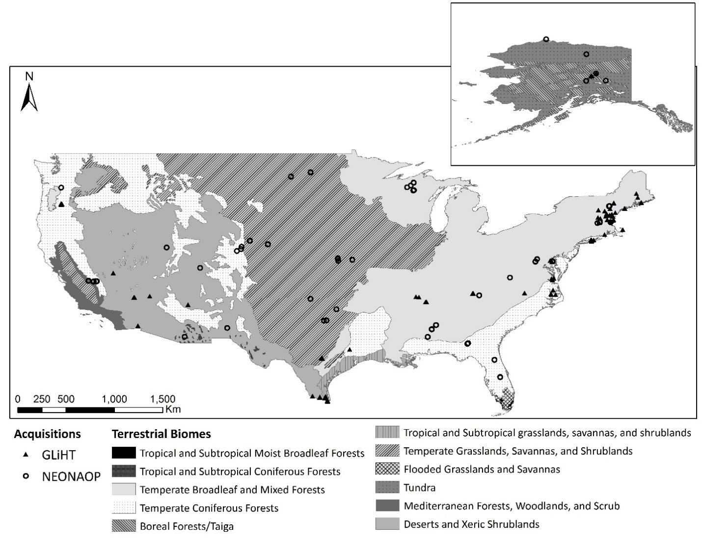
Figure 2. Locations of LiDAR acquisitions overlaid on 11 terrestrial biomes of the conterminous U.S. and Alaska (as defined by Olson et al., 2001).
Landsat Imagery
: Landsat Collection-1 SR images (Landsat 8 Operational Land Imager (OLI)/Thermal Infrared Sensor (TIRS), Landsat 7 Enhanced Thematic Mapper Plus (ETM+), and Landsat 4-5 Thematic Mapper (TM)) were downloaded from the U.S. Geological Survey (USGS) Earth Resources Observation and Science Center (EROS) (https://www.usgs.gov/centers/eros/). These images included the scenes overlapping the LiDAR acquisitions, and the 443 path-row scenes that span the conterminous U.S. for the majority of the Landsat archive data (1984–2018). Only the visible (V) bands (blue, red, and green), near infrared (NIR), and the two short-wave infrared (SWIR1 and SWIR2) bands were used in the analysis. The Landsat images, the resulting rasters from the LiDAR data, and the SR data were processed using the R software (R Core Team, 2018).
Training & Validation Dataset Construction
To construct the fractional cover models, a training and validation dataset was produced with a 30 m spatial resolution that included four response variables derived from the LiDAR/multispectral data (percent trees, percent shrub, percent herb, percent other), six predictor variables derived from the Landsat SR data (Blue, Red, Green, Near Infrared, Short-wave Infrared 1, and Short-wave Infrared 2), and a categorical variable defined as the biome-cover stratum used for separating the data into training and validation: this variable was constructed by concatenating the number of the terrestrial biome corresponding to each acquisition, and the numbers resulting from classifying each lifeform percent cover into quantile classes (i.e. 0%-25%, 25%-50%, 50%-75%, and 75%-100%).
Lifeform Classes
The differentiation of lifeform classes was based on a) the vertical structure of the vegetation derived from the LiDAR data, and b) an index derived from SR data to separate live vegetation from non-vegetation or dead vegetation features (hereafter referred to as “non-vegetation”). Height thresholds were first defined for separating tree, shrub, and herb lifeforms based on an evaluation of different published classification systems and previous works on the construction of continuous fields maps (Anderson et al., 1976; Dansereau, 1951; DeFries et al., 1999; Di Gregorio and Jansen 2000; Hansen et al., 2013; Sexton et al., 2013; Xian et al., 2015). Based on these references, the LiDAR-based canopy height models (CHM) were classified into three separate layers a) features <0.5 m in height (herb), b) features >=0.5 m and <5 m high (shrub), and c) features >= 5 m high (tree). Normalized Difference Vegetation Index (NDVI) (Tucker, 1979) from each SR acquisition was used to differentiate live vegetation from non-vegetation using a simple threshold value. To determine the threshold, NEON acquisitions were used that had available orthophotos (13 used in total). Two NEON sites were randomly selected from each of the terrestrial biomes to have an equal representation of biomes with different characteristics (Table 3).
Table 4. NEON sites used for NDVI threshold selection.
| Site ID | Site Name | Year of Acquisition | Terrestrial Biome |
|---|---|---|---|
| DEJU | Delta Junction | 2017 | Boreal Forests/Taiga |
| SRER | Santa Rita Experimental Range | 2017 | Deserts and Xeric Shrublands |
| JORN | Jornada LTER | 2017 | Deserts and Xeric Shrublands |
| SJER | San Joaquin Experimental Range | 2013; 2017 | Mediterranean Forests, Woodlands, and Scrub |
| GRSM | Great Smoky Mountains National Park, Twin Creeks | 2015 | Temperate Broadleaf and Mixed Forests |
| DELA | Dead Lake | 2016 | Temperate Broadleaf and Mixed Forests |
| DSNY | Disney Wilderness Preserve | 2014 | Temperate Coniferous Forests |
| RMNP | Rocky Mountain National Park | 2017 | Temperate Coniferous Forests |
| UKFS | The University of Kansas Field Station | 2017 | Temperate Grasslands, Savannas, and Shrublands |
| OAES | Klemme Range Research Station | 2017 | Temperate Grasslands, Savannas, and Shrublands |
| BONA | Caribou-Poker Creeks Research Watershed | 2017 | Tundra |
| BARR | Barrow Environmental Observatory | 2017 | Tundra |
Other (non-vegetation) Class
The orthophotos of each selected site were mosaicked, and a shapefile of 100 random points was created for each acquisition. Each point was photo interpreted and classified into live vegetation and non-vegetation. The NDVI value for each point was extracted from the correspondent NDVI raster for each year and acquisition site. A beta distribution was fitted to the NDVI data of the live vegetation features, and a truncated lognormal distribution to the non-vegetation feature class. The 10% quantile of the live vegetation distribution and 90% quantile of the non-vegetation distribution were calculated to inform the final NDVI threshold value of 0.42 which was used to classify each NDVI raster pixel into live vegetation or non-vegetation.
Landsat SR
The classification of each acquisition site into tree, shrub, herb, and other, was done by merging the classified NDVI and CHM layers, such that Other corresponded to all the features that are non-vegetation, regardless of their height, while herb, shrub, and tree correspond to live vegetation features below 0.5 m, between 0.5 m and 5 m, and above 5 m respectively. The resulting lifeform rasters were paired with a corresponding SR Landsat scene. Images with the least possible cloud cover within a month from the orthophoto acquisition date were selected, and the V/NIR/SWIR bands of the Landsat scenes were included in the analysis. Each Landsat scene was masked to remove non-clear pixels (pixels with cloud, water, ice, snow, or cloud shadow cover) and cropped using the acquisition’s bounding box. The final lifeform rasters were aligned to each Landsat cropped scene, resampled to a 30-m pixel resolution, stacked with the cropped SR Landsat bands, and transformed into a database.
Landsat pixels that were not completely covered by the lifeform rasters, commonly occurring at the edge of the LiDAR acquisition area, were removed from the dataset. The resulting data from all the available acquisitions were merged into a single dataset. To guarantee an equal representation of different biomes and lifeform cover conditions in the final training data, two classification IDs were included in the dataset: the terrestrial biome classification ID derived from the Terrestrial Ecoregions of the World map (Olson et al., 2001), and the cover ID. This last ID was constructed by classifying percent cover values of each lifeform into one of four categories and combining the resulting numbers in a unique ID; cover values between 0–25% were labeled as one, 25–50% were labeled as two, 50–75% corresponded to three, and values over 75% corresponded to four.
Combined LiDAR/Multispectral Dataset
The combined dataset had an N=9,990,526. The data were divided into training and validation subsets and to guarantee equal representation of the different cover ID classes and of the different biomes in the training data, the same number of samples was drawn from each cover ID class. Furthermore, the number of samples was divided equally among the available Biome ID nested in each cover ID class. If a specific ID class did not have the number of samples required for the training dataset, the available data were upsampled by resampling with replacement.
Lifeform Regression Models
A quantile regression forests model was constructed with the training data for each of the lifeform cover types using the R (R Core Team, 2018) package quantregForest (Meinshausen, 2017). To assess performance and uncertainty, predicted values were compared to validation data at overlapping locations (Table 2). Mean prediction values for each of the lifeform cover types were estimated as well as a prediction interval which was used to evaluate the spatially explicit uncertainty of the prediction values. An overview of the model construction workflow is presented in Figure 3.
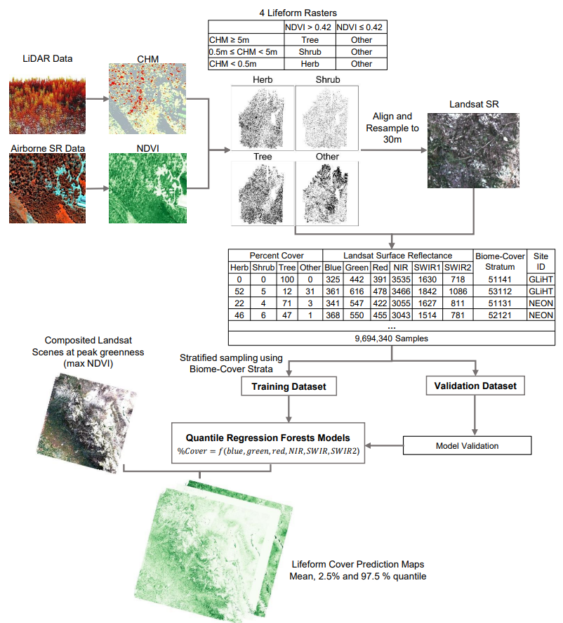
Figure 3. Lifeform cover models construction workflow.
Data Access
These data are available through the Oak Ridge National Laboratory (ORNL) Distributed Active Archive Center (DAAC).
CMS: Vegetative Lifeform Cover from Landsat SR for CONUS, 1984-2018
Contact for Data Center Access Information:
- E-mail: uso@daac.ornl.gov
- Telephone: +1 (865) 241-3952
References
Anderson, J.R., E.E. Hardy, J.T. Roach, and R.E. Witmer. 1976. A Land Use and Land Cover Classification System for Use with Remote Sensor Data. US Geological Survey, Professional Paper 964. USGS Publications Warehouse; Washington, D.C. https://doi.org/10.3133/pp964
Cook, B., L. Corp, R. Nelson, E. Middleton, D. Morton, J. McCorkel, J. Masek, K. Ranson, V. Ly, and P. Montesano. 2013. NASA Goddard’s LiDAR, Hyperspectral and Thermal (G-LiHT) Airborne Imager. Remote Sensing 5:4045–4066. https://doi.org/doi:10.3390/rs5084045
Dansereau, P. 1951. Description and recording of vegetation upon a structural basis. Ecology 32:172–229. https://doi.org/10.2307/1930415
DeFries, R.S., J.R.G. Townshend, and M.C. Hansen. 1999. Continuous fields of vegetation characteristics at the global scale at 1-km resolution. Journal of Geophysical Research: Atmospheres 104:16911–16923. https://doi.org/10.1029/1999JD900057
Di Gregorio, A. and L.J.M. Jansen. 2000. Land Cover Classification System (LCCS). Classification Concepts and User Manual. Food and Agriculture Organization of the United Nations (FAO); Rome, Italy. https://www.fao.org/3/x0596e/x0596e00.htm
Hansen, M.C., P.V. Potapov, R. Moore, M. Hancher, S.A. Turubanova, A. Tyukavina, D. Thau, S.V. Stehman, S.J. Goetz, T.R. Loveland, A. Kommareddy, A. Egorov, L. Chini, C.O. Justice, and J.R.G. Townshend. 2013. High-resolution global maps of 21st-Century forest cover change. Science 342:850–853. https://doi.org/10.1126/science.1244693
Meinshausen, N. 2017. QuantregForest: Quantile Regression Forests. https://cran.r-project.org/web/packages/quantregForest/quantregForest.pdf
NEON. 2017. Provisional Data. Downloaded on July 2017. Battelle, Boulder, CO, USA. https://www.neonscience.org/data-collection/airborne-remote-sensing
Olson, D.M., E. Dinerstein, E.D. Wikramanayake, N.D. Burgess, G.V.N. Powell, E.C. Underwood, J.A. D’amico, I. Itoua, H.E. Strand, J.C. Morrison, C.J. Loucks, T.F. Allnutt, T.H. Ricketts, Y. Kura, J.F. Lamoreux, W.W. Wettengel, P. Hedao, and K.R. Kassem.. 2001. Terrestrial Ecoregions of the World: A New Map of Life on Earth. BioScience 51: 933-938. https://doi.org/10.1641/0006-3568(2001)051[0933:TEOTWA]2.0.CO;2
A. Parra and J. A. Greenberg, "Estimation of Fractional Plant Lifeform Cover for the Conterminous United States Using Landsat Imagery and Airborne LiDAR," in IEEE Transactions on Geoscience and Remote Sensing, vol. 60, pp. 1-14, 2022, Art no. 4413614, doi: 10.1109/TGRS.2022.3199156
R Core Team. 2018. R: A Language and Environment for Statistical Computing. Vienna, Austria: R Foundation for Statistical Computing. https://www.r-project.org
Sexton, J.O., X.-P. Song, M. Feng, P. Noojipady, A. Anand, C. Huang, D.-H. Kim, K.M. Collins, S. Channan, C. DiMiceli, and J.R. Townshend. 2013. Global, 30-m resolution continuous fields of tree cover: Landsat-based rescaling of MODIS vegetation continuous fields with lidar-based estimates of error. International Journal of Digital Earth 6:427–448. https://doi.org/10.1080/17538947.2013.786146
Tucker, C.J. 1979. Red and photographic infrared linear combinations for monitoring vegetation. Remote Sensing of Environment 8:127–150. https://doi.org/10.1016/0034-4257(79)90013-0
Xian, G., C. Homer, M. Rigge, H. Shi, and D. Meyer. 2015. Characterization of shrubland ecosystem components as continuous fields in the northwest United States. Remote Sensing of Environment 168:286–300. https://doi.org/10.1016/j.rse.2015.07.014