Documentation Revision Date: 2020-04-06
Dataset Version: 1
Summary
There are eight files in GeoTIFF (.tif) format with the SOC estimates and uncertainties and two files in comma-separated (.csv) format with this data set. The .csv files contain the calculated SOC stock for each soil sample point.
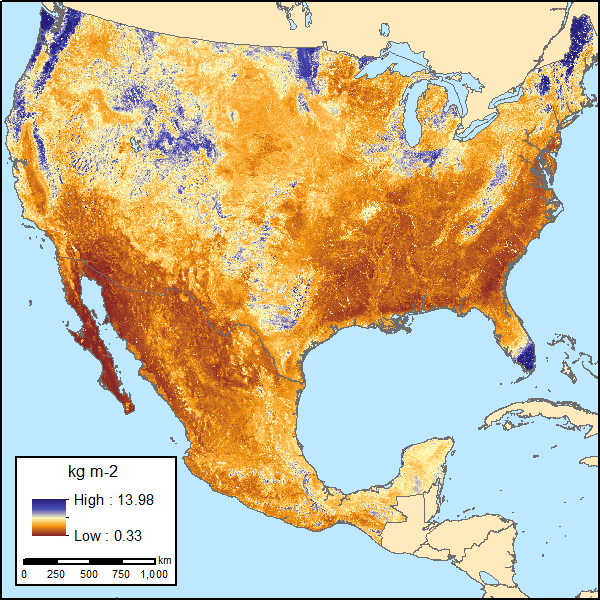
Figure 1. Soil organic carbon (SOC) for 0-30 cm topsoil layer in kg SOC/m2 at 250-m resolution across Mexico and the conterminous USA (CONUS) for the period 1991-2010. Source: data file SOC_prediction_1991_2010.tif
Citation
Guevara, M., C.E. Arroyo-cruz, N. Brunsell, C.O. Cruz-gaistardo, G.M. Domke, J. Equihua, J. Etchevers, D.J. Hayes, T. Hengl, A. Ibelles, K. Johnson, B. de Jong, Z. Libohova, R. Llamas, L. Nave, J.L. Ornelas, F. Paz, R. Ressl, A. Schwartz, S. Wills, and R. Vargas. 2020. Soil Organic Carbon Estimates for 30-cm Depth, Mexico and Conterminous USA, 1991-2011. ORNL DAAC, Oak Ridge, Tennessee, USA. https://doi.org/10.3334/ORNLDAAC/1737
Table of Contents
- Dataset Overview
- Data Characteristics
- Application and Derivation
- Quality Assessment
- Data Acquisition, Materials, and Methods
- Data Access
- References
Dataset Overview
This dataset provides two sets of gridded estimates of estimated soil organic carbon (SOC) and associated uncertainties for 0-30 cm topsoil layer in kg SOC/m2 at 250-m resolution across Mexico and the conterminous USA (CONUS). The first set of estimates, for the period 1991-2010, were derived using multi-source SOC field data and multiple environmental variables representative of the soil forming environment coupled with a machine learning approach (i.e., simulated annealing) and regression tree ensemble modeling for optimized SOC prediction. Predictions of gridded SOC and uncertainty based on multiple bulk density (BD) pedotransfer functions (PTFs) are also included. The second set of estimates, for the period 2009-2011, were derived from two fully independent validation field datasets from across both countries. Note that the same environmental variables and modeling approach used for the first set of estimates were applied to the second set to assess the models' sensitivity to multiple SOC data sources. The SOC field data for the first set of estimates are provided in this dataset and the other data sources, including the two independent validation field datasets, are referenced.
Project: Carbon Monitoring System (CMS)
The NASA Carbon Monitoring System (CMS) is designed to make significant contributions in characterizing, quantifying, understanding, and predicting the evolution of global carbon sources and sinks through improved monitoring of carbon stocks and fluxes. The System will use the full range of NASA satellite observations and modeling/analysis capabilities to establish the accuracy, quantitative uncertainties, and utility of products for supporting national and international policy, regulatory, and management activities. CMS will maintain a global emphasis while providing finer scale regional information, utilizing space-based and surface-based data and will rapidly initiate generation and distribution of products both for user evaluation and to inform near-term policy development and planning.
Related Dataset:
Guevara, M., and R. Vargas. 2020. Soil Organic Carbon Estimates and Uncertainty for 1-m Depth across Mexico, 1999-2009. ORNL DAAC, Oak Ridge, Tennessee, USA. https://doi.org/10.3334/ORNLDAAC/1754
Related Publication:
Guevara, M., C. Arroyo, N. Brunsell, C.O. Cruz, G. Domke, J. Equihua, J. Etchevers, D. Hayes, T. Hengl, A. Ibelles, K. Johnson, B. de Jong, Z. Libohova, R. Llamas, L. Nave, J.L. Ornelas, F. Paz, R. Ressl, A. Schwartz, A. Victoria, S. Wills and R. Vargas. 2020. Soil Organic Carbon across Mexico and the conterminous United States (1991-2010). Global Biogeochemical Cycles, 34, e2019GB006219. https://doi.org/10.1029/2019GB006219
Acknowledgement:
This study was supported by NASA’s Carbon Monitoring System Program under grant number 80NSSC18K0173.
Data Characteristics
Spatial Coverage: Mexico and the conterminous USA (CONUS)
Spatial Resolution: 250 m
Temporal Coverage: 1991-01-01 to 2011-12-31
Temporal Resolution: One-time SOC model predictions
Study Areas (All latitude and longitude given in decimal degrees)
|
Sites |
Westernmost Longitude |
Easternmost Longitude |
Northernmost Latitude |
Southernmost Latitude |
|---|---|---|---|---|
|
CONUS and Mexico |
-129.7893167 |
-65.57936389 |
49.61068333 |
11.32335833 |
Data File Information
This dataset includes eight data files in GeoTIFF (.tif) format at 250-m resolution and two files in comma-separated format (.csv).
Table 1. File names and descriptions
| File Names | Descriptions |
|---|---|
|
SOC_prediction_1991_2000.tif |
Gridded SOC prediction (250m) across CONUS and Mexico using ISCN and INEGI SOC observations collected between 1991-2000 as training data |
|
SOC_prediction_2001_2010.tif |
Gridded SOC prediction (250m) across CONUS and Mexico using ISCN and INEGI SOC observations collected between 2001-2010 as training data |
|
SOC_prediction_1991_2010.tif |
Gridded SOC prediction (250 m) across CONUS and Mexico using ISCN and INEGI SOC observations collected between 1991-2010 as training data |
|
prediction_limits_bulk_density_pedotransfer.tif |
Range of prediction limits based on multiple BD pedotransfer functions, 1991-2010 |
|
SOC_uncertainty_bulk_density_pedotransfer.tif |
SOC uncertainty associated with the variance of multiple BD pedotransfer functions, 1991-2010 |
|
SOC_prediction_independent_dataset.tif |
Gridded SOC prediction in CONUS and Mexico using RaCA and INFyS SOC observations collected in 2009-2011 as training data Note the purpose of this set of SOC prediction was used for validating the sensitivity of models developed in Guevara et al., 2020 |
|
prediction_limits_independent_dataset.tif |
Range of prediction limits based on independent datasets used for validation, 2009-2011 |
|
SOC_uncertainty_independent_dataset.tif |
SOC uncertainty associated with independent datasets used for validation, 2009-2011 |
|
ISCN_INEGI_SOC_stocks_1991_2010.csv |
SOC data and collection information from the ISCN and the INEGI used for calculating SOC stock estimates |
|
wosis_SOC_bulk_density_pedotransfer_1991_2010.csv |
SOC based on the six bulk density functions and mean errors |
GeoTIFF files
The eight maps have a spatial resolution of 250 m and represent SOC related variables in kg/SOC/m2.
Coordinate Reference System:
The geographic information is provided in 250-m grids in a custom azimuthal equidistant projection. Use this proj4 spatial reference code for processing.
' +proj=aeqd +lat_0=52 +lon_0=-97.5 +x_0=8264722.17686 +y_0=4867518.35323 +datum=WGS84 +units=m +no_defs +ellps=WGS84 +towgs84=0,0,0'
Band: single
No data value: -9999
Map units: meters
Table 2. Variables in the file ISCN_INEGI_SOC_stocks_1991_2010.csv
| Variable | Description |
|---|---|
| x | X coordinate in a custom azimuthal equidistant projection |
| y | Y coordinate in a custom azimuthal equidistant projection |
| soc | SOC content in kg/SOC/m2 |
| period | Time period of data (i.e. “1991-2000” or “2001-2010”) |
| src | Source of base information for calculating SOC stocks (INEGI and ISCN) |
Table 3. Variables in the file wosis_SOC_bulk_density_pedotransfer_1991_2010.csv
SOC content in kg/SOC/m2
Error* of SOC based on bulk density function of Drew (1973)
| Variable | Description |
|---|---|
| x | X coordinate in a custom azimuthal equidistant projection |
| y | Y coordinate in a custom azimuthal equidistant projection |
| period | Period of time of data (i.e. “1991-2000” or “2001-2010”) |
| src | Source of base information for calculating SOC stocks (WoSIS) |
| soc_saini | SOC based on bulk density function of Saini (1966) |
| soc_drew | SOC based on bulk density function of Drew (1973) |
| soc_grigal | SOC based on bulk density function of Grigal et al. (1989) |
| soc_jeffrey | SOC based on bulk density function of Jeffrey (1970) |
| soc_madams | SOC based on bulk density function of Adams (1973) |
| soc_mhoney | SOC based on bulk density function of Honeysett and Ratkowsky (1989) |
| mean_error_saini | Error* of SOC based on bulk density function of Saini (1966) |
| mean_error_drew | Error* of SOC based on bulk density function of Drew (1973) |
| mean_error_grigal | Error* of SOC based on bulk density function of Grigal et al. (1989) |
| mean_error_jeffrey | Error* of SOC based on bulk density function of Jeffrey (1970) |
| mean_error_adams | Error* of SOC based on bulk density function of Adams (1973) |
| mean_error_honeysett | Error* of SOC based on bulk density function of Honeysett and Ratkowsky (1989) |
* These errors were calculated using Taylor series as implemented in the OCSKGM function of the GSIF package of R for statistical computing.
Application and Derivation
Soil Organic Carbon (SOC) information is fundamental for improving global carbon cycle modeling efforts. These data provide context for estimates based on SOC legacy data and benchmarks for improving regional-to-global monitoring efforts (Guevara et al., 2020).
Additional Usage Guidance Provided by the Authors
Q: Which file would you suggest users to use if they want to reuse your SOC predictions in their own study?
A: The model for the period 1991-2010 (SOC_prediction_1991_2010.tif ) is recommended as baseline for further general applications because it relies on the major number of observations for training. This is the target period of time selected for this study and the associated maps 1991-2000, 2001-2010 should be seen as complementary.
Q: What are the potential uses of the 1991-2000 and 2001-2010 maps (SOC_prediction_1991_2000.tif and SOC_prediction_2001_2010.tif)?
A: The maps 1991-2000 and 2001-2010 were produced to extract additional information on the prediction variance associated with differences in SOC inventories.
Further work could be focused on using these maps as benchmarks for both modeling efficiency, differences in methodologies and potential SOC changes. We clarify that the 1991-2000 and 2001-2010 maps do not represent absolute differences in SOC between the time-periods, as uncertainties in these estimates must be taken into account. Thus, we recommend that users do not use the absolute values of these 1991-2000 and 2001-2010 maps to calculate absolute SOC differences between these periods without taken into consideration uncertainties.
Q: Which map should I use for more recent SOC data?
A: We provide a map representing the period between 2009 and 2011 (SOC_prediction_independent_dataset.tif) (RaCA and INFyS) and analyze the variance against the aforementioned (ISCN and INEGI) SOC predictions (Fig. 7 in Guevara et al., 2020) striving to quantify the spatial variability of SOC. This map (RaCA and INFyS) could be useful for some user specific needs requiring ‘more recent’ SOC data and users that may be concerned about using "legacy data" (e.g., < 2000).
Q: How did you use the SOC predictions using independent observations to validate your 3 sets of SOC predictions using the ISCN and INEGI SOC observations? The independent observations were in 2009-2011, while your other 3 SOC predictions represent different time frames.
A: Each model has its own internal cross-validation with the training data, but we also compared model outputs using different SOC inventories. The underlying assumption for comparing SOC predictions based on different time frames is that SOC stocks and associated spatial variability is comparable among decades/datasets (e.g., 1991-2010 and 2009-2011). We highlight that uncertainty in model predictions are larger than potential real SOC differences. We understand that this may be controversial but is the conclusion that our research shows when upscaling SOC estimates across North America using different decades/datasets (Guevara et al., 2020).
For example, we calculate and compare SOC stocks from both maps (~46 Pg predicted with the ISCN-INEGI 1991-2010 data to 47 Pg predicted with the RaCA and INFyS data). Higher discrepancy (from 44 to 55 Pg) was found when limiting training data to one decade (independent models for the years 1991-2000 and for the years 2001-2010), probably associated with underrepresented areas with no data for one decade (1991-2000) or the other (2001-2010).
The use of SOC data from multiple periods of time is common on baseline SOC mapping efforts due to limited data availability, in order to increase spatial representativeness while compromising temporal resolution.
Q: How did you convert the discrete 1) residual variances of model prediction against 6 PDBD SOC estimates and 2) residual of model prediction against independent prediction onto a 250-m grid?
A: We used a geostatistical approach (Ordinary Kriging) to quantify the spatial structure of modeling errors (the relation between variance of values and distance between locations where these values are collected defined by latitude and longitude coordinates) (see Fig. 4 in Guevara et al., 2020). As explained by previous work on soil predictive mapping (e.g., References 1 and 2), the universal model of soil variation suggest that soil variation could be analyzed as the combined result of:
1) a deterministic component (e.g., based on the expected relationships (linear and nonlinear) between soil-target variables and the soil forming environment),
2) plus, an error that is spatially autocorrelated (The errors in Fig. 6 of Guevara et al., 2020.) and that can then provide additional information in the spatial pattern of the soil target variable, and
3) plus, ‘pure noise’ or uncorrelated components of variability beyond the resolution of the method (or set of methods) used by the soil surveyor for collecting and analyzing soil samples (e.g., errors in coordinates). In short: soil variation=deterministic component + spatially autocorrelated error + pure noise).
We analyzed these three components of the universal model of soil variation using:
1) a tree-based regression model assuming a deterministic relationship between SOC data (field data) and the covariates selected by the simulated annealing framework, (see section 3.3 of Guevara et al., 2020) to represent soil forming factors.
2) We used Geostatistics for analyzing the spatial structure of residual errors (Fig. 4 of Guevara et al., 2020). Geostatistics relies on variogram analysis for quantifying the spatial structure of target variables (at the locations where they are measured) in the geographical space of a complete area of interest.
3) We also used the variogram to calculate the uncorrelated component of soil variation given available data (known in Geostatistics as ‘nugget effect’).
We did find spatial structure in modeling residuals (Fig. 4 of Guevara et al., 2020) and therefore proceeded with the Kriging analysis to interpolate errors in order to provide spatially distributed and contiguous surrogates of uncertainty (Fig. 6 of Guevara et al., 2020); associated with both a) the bulk density pedotransfer functions and b) with the use of slightly more recent datasets (RaCA INFyS) representative of a shorter period of time. These analyses were performed using automated automatic variogram fitting. The variogram fitting and the interpolation of errors via Kriging was performed using the package of R ‘automap’ (developed for previous applications, Reference 3).
Application References:
1-Burrough, P. A., and R. A. McDonnell. 1998. Principles of Geographical Information Systems. 2nd ed. Oxford: Oxford University Press.
2-Webster, R., and M.A. Oliver. 2001. Geostatistics for Environmental Scientists. Statistics in Practice. Chichester: Wiley.
3- Hiemstra, P. H., Pebesma, E. J., Twenhöfel, C. J. W. and Heuvelink, G. B. M.: Real-time automatic interpolation of ambient gamma dose rates from the Dutch radioactivity monitoring network, Computers & Geosciences, 35(8), 1711–1721, doi:10.1016/j.cageo.2008.10.011, 2009.
Q: Is there a common identifier (or a key) column to associate records between these two CSV files: ISCN_INEGI_SOC_stocks_1991_2010.csv and wosis_SOC_bulk_density_pedotransfer_1991_2010.csv ?
A: We have not included a spatial analysis and generated a unique spatial ID, but the spatial coordinates (i.e., latitude, longitude) are included in both datasets. This decision was taken because WoSIS has its own quality control protocol (including IDs) and renaming samples may cause confusion if further efforts would like to merge our dataset with WoSIS. We believe that spatial coordinates may be sufficient for identification and would simplify the dataset. Future work could be focused on identifying the precise link between these multiple sources of SOC data and their associated locations with registered IDs within WoSIS or expand it.
Quality Assessment
The residual variance of six conventional pedotransfer functions for estimating bulk density to calculate SOC stocks was analyzed. The mean errors are provided with this dataset. Two independent SOC datasets confirmed that the SOC stock for both countries are between 46 and 47 Pg. When reducing training data to arbitrary defined decades (1991-2000 and 2001-2010, respectively), model sensitivities for predicted SOC stocks ranged between 41 and 55 Pg (Guevara et al., 2020).
Data Acquisition, Materials, and Methods
The spatial distribution of SOC stocks (topsoil; 0-30 cm) across Mexico and the conterminous US (CONUS) was modeled and the uncertainty was quantified. A digital soil mapping strategy was followed for the prediction of the spatial variability of SOC across both countries.
Following is a brief synopsis of the methods found in Guevara et al. (2020).
SOC Observational Data
Sources:
- Legacy SOC estimates across CONUS were obtained from the International Soil Carbon Network (ISCN latest version 2018, >18,000 pedons available, Harden et al., 2017).
- Data from Mexico were provided by the Instituto Nacional de Estadística y Geografía (INEGI, SERIES 1 & 2; n >65,000 pedons available, Krasilnikov et al., 2013).
- Only observations collected between 1991 and 2010 were used to minimize confounding factors (related to potential changes in the SOC pool; n = 10,385.
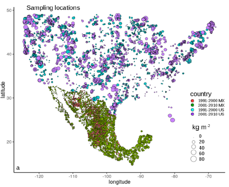
Figure 2. Point map showing the spatial distribution of sampling locations and the calculated SOC content in the first 30 cm soil from available data for the period 1991-2010 (1991-2000 and 2001-2010) (Guevara et al. (2020)).
Processing:
The combination of using soil depth continuous functions (Bishop et al., 1999; Malone et al., 2009) and deriving the weighted average (by depth) from the first sampled soil horizon at 0 cm depth to all soil horizons sampled within the first 30 cm of soil depth, allowed aggregating irregular soil horizons for calculating SOC stocks across both countries. The weights for calculating these stocks were selected defining the proportion of each horizon within this 0-30 cm interval of soil depth.
Most contributors (across CONUS) and INEGI (in Mexico) considered (or adapted) the United States Department of Agriculture Soil Taxonomy guidelines for interpreting soil surveys including SOC and other soil variables (Soil Survey Staff. 1999). For CONUS, the ISCN database provides a harmonized compilation from many contributors (e.g., Natural Resources Conservation Service, United States Geological Survey and site-specific research or academic groups; Harden et al., 2017). However, the largest contributor for this curated dataset is the United States Department of Agriculture Natural Resource Conservation Service, where the SOC concentration was mainly obtained by the Walkley-Black technique (Soil Survey Staff. 2014). All samples for Mexico were systematically collected and analyzed by INEGI (INEGI, 2014, Krasilnikov et al., 2013) and SOC concentration was also measured using the Walkley-Black technique (IUSS-WRB-FAO, 2014).
Calculation of SOC Stocks
SOC stocks were derived by a linear combination of soil depth (0-30cm), coarse fragments (CF) data, SOC concentration (%), and soil bulk density (BD) as implemented by Hengl (2017).
- For the CONUS dataset, the ISCN has calculated SOC stocks using both modeled (i.e., incomplete) and non-modeled (i.e., complete) information about the aforementioned variables (Harden et al. 2017). Only information flagged as ‘complete’ by the ISCN was used, so no model or pedotransfer functions were used for estimating BD and consequently SOC stocks.
- In Mexico, BD was estimated in the field using soil type maps, soil texture, soil organic matter and soil structure following international soil mapping guidelines (FAO, 2006, p 51, Table 58).
Environmental Covariates
Environmental covariates used were from the SoilGrids 250m system (Hengl et al., 2017). This covariate space is representative for the analyzed period of time (1991-2010). This global information was extracted within the geographical limits of the NALCMS (North American Land change Monitoring System, 77% of land use classification accuracy) at 250 m spatial resolution (NRCan/CCRS-USGS-INEGI-CONABIO-CONAFOR, 2010).
Recursive Feature Elimination
A variable reduction strategy was performed using a recursive feature elimination technique (Kuhn et al., 2008) and multiple models were fitted repeatedly using all possible combinations of highly ranked predictors. After a 5-times repeated 5-fold cross validation for the recursive feature elimination technique (to account for the model sensitivity to data variations and reduce overfitting), the first 25 environmental covariates for SOC were selected. A simulated annealing framework was applied to maximize the feature selection and prediction accuracy of SOC relevant environmental covariates. The Random Forest regression algorithm within the simulated annealing framework was used to improve the probability of detecting the main drivers of SOC spatial patterns. After a 5-times repeated 5-fold cross validation, the entire data set was used for generating a model in the last execution of the simulated annealing global search.
Uncertainty Analysis and Pedotransfer Functions for Bulk Density Variance
The uncertainty of the modeling approach was represented as the sensitivity of prediction models to multiple data inputs. SOC stocks were predicted at the pedon locations available in the WoSIS system (Batjes et al., 2016). The residual variance of the predictions and independent SOC stocks were calculated. Independent stocks were calculated using the WoSIS SOC concentration data (%), and six conventional pedotransfer functions for estimating BD. This resulted in six different SOC stocks estimates from the following pedotransfer functions:
|
Saini (1966): BD = 1.62 - 0.06 * OM , Jeffrey (1970): BD = 1.482 - 0.6786 * (log(OM)) |
|
Jeffrey (1970): BD = 1.482 - 0.6786 * (log(OM)) |
|
Adams (1973): = 100 / (OM /0.244 + (100 - OM)/2.65) |
|
Drew (1973): BD = 1 / (0.6268 + 0.0361 * OM) |
|
Honeysett & Ratkowsky (1989): BD = 1/(0.564 + 0.0556 * OM) |
|
Grigal et al. (1989): BD = 0.669 + 0.941 * exp(1)^(-0.06 * OM) |
| Note: The OM= organic matter content was estimated as OM=SOC concentration * 1.724. |
These functions applied to the WoSIS data were selected because they were developed for a variety of soil weathering environments using multiple analytical techniques for measuring SOC and because they were recently proposed for the development of the United Nations global SOC map (Yigini et al., 2018). In addition, the WoSIS data has been curated under different protocols for controlling data quality and global interoperability standards (Batjes et al. 2017) and thus, this residual variance will allow us to have an idea of possible dispersion of values around the SOC calculated stocks.
Independent Datasets for Model Prediction
Gridded estimates of SOC and uncertainties were also derived from two fully independent field datasets from across both countries. The same simulated annealing framework and modeling approaches were applied to the independent datasets.
These independent datasets were collected using different sampling designs and using different SOC calculation methods from our initial training dataset (INEGI and ISCN). Across CONUS, 6,179 SOC estimates (2010) were used from the Rapid Carbon Assessment Project (RaCA, Soil Survey Staff and Loecke, 2016; Wijewardane et al., 2017), and 3,060 (2009-2011). SOC estimates were used from topsoil samples extracted from the Mexican National Forest and Soils Inventory of the Mexican Forest Service.
Model residuals were calculated against two fully independent datasets across both countries (n=9239).
The residual analysis against these independent datasets provided an overall measure of the models’ sensitivity to multiple SOC data sources as described in Guevara et al. (2020).
Data Access
These data are available through the Oak Ridge National Laboratory (ORNL) Distributed Active Archive Center (DAAC).
Soil Organic Carbon Estimates for 30-cm Depth, Mexico and Conterminous USA, 1991-2011
Contact for Data Center Access Information:
- E-mail: uso@daac.ornl.gov
- Telephone: +1 (865) 241-3952
References
Adams, W.A. (1973). The effect of organic matter on the bulk and true densities of some uncultivated podzolic soils. European Journal of Soil Science, 24(1):10–17.https://doi.org/10.1111/j.1365-2389.1973.tb00737.x
Batjes, N.H. (2016). Harmonized soil property values for broad-scale modelling (WISE30sec) with estimates of global soil carbon stocks. Geoderma, 269, 61–68. https://doi.org/10.1016/j.geoderma.2016.01.034
Batjes NH, Ribeiro E, van Oostrum A, Leenaars J, Hengl T, Mendes de Jesus J (2017) WoSIS:providing standardised soil profile data for the world. Earth System Science Data, 9, 1–14. https://doi.org/10.5194/essd-9-1-2017
Bishop TFA, McBratney AB, Laslett GM (1999) Modelling soil attribute depth functions with equal area quadratic smoothing splines. Geoderma, 91, 27–45. https://doi.org/10.1016/S0016-7061(99)00003-8
Drew, L. A.: (1973) Bulk Density Estimation Based on Organic Matter Content of Some Minnesota Soils, St. Paul, Minn., School of Forestry, University of Minnesota, Digital Conservancy, available at: http://hdl.handle.net/11299/58293
FAO 2017. Soil Organic Carbon: the hidden potential. Food and Agriculture Organization of the United Nations, Rome, Italy.
FAO Guidelines for soil description Fourth edition, Rome 2006 109 pp. FAO and ITPS. 2018. Global Soil Organic Carbon Map (GSOCmap) Technical Report. Rome. 162 pp.
FAO and ITPS. 2018. Global Soil Organic Carbon Map (GSOCmap) Technical Report. Rome. 162pp.
Grigal, D.,S. Brovold, W. Nord, and L. Ohmann. (1989). Bulk density of surface soils and peat in the north central united states. Canadian Journal of Soil Science, 69(4):895–900. http://dx.doi.org/10.4141/cjss89-092
Guevara, M., C. Arroyo, N. Brunsell, C.O. Cruz, G. Domke, J. Equihua, J. Etchevers, D. Hayes, T. Hengl, A. Ibelles, K. Johnson, B. de Jong, Z. Libohova, R. Llamas, L. Nave, J.L. Ornelas, F. Paz, R. Ressl, A. Schwartz, A. Victoria, S. Wills and R. Vargas. 2020. Soil Organic Carbon across Mexico and the conterminous United States (1991-2010). Global Biogeochemical Cycles, 34, e2019GB006219. https://doi.org/10.1029/2019GB006219
Harden, J.W., G. Hugelius, A. Ahlström, et al. (2018). Networking our science to characterize the state, vulnerabilities, and management opportunities of soil organic matter. Global Change Biology, Feb;24(2):e705-e718. https://doi.org/10.1111/gcb.13896
Hengl, T. (2017). GSIF: Global Soil Information Facilities. R package version 0.5-1. https://CRAN.R- project.org/package=GSIF
Hengl T, Mendes J, Heuvelink GBM, et al. (2017) SoilGrids250m: global gridded soil information based on Machine Learning. PLoS ONE 12(2): e0169748.https://doi.org/10.1371/journal.pone.0169748
Honeysett, J. and D. Ratkowsky. (1989). The use of ignition loss to estimate bulk density of forest soils. European Journal of Soil Science, 40(2):299–308. https://doi.org/10.1111/j.1365-2389.1989.tb01275.x.
INEGI-Instituto Nagional de Geografia y Estadistica (2014) Diccionario de Datos Edafológicos escala 1:250000 (version 3) 55pp. http://www.inegi.org.mx/geo/contenidos/recnat/edafologia/doc/dd_edafologicos_v3_250k.pdf
Jeffrey, D. (1970). A note on the use of ignition loss as a means for the approximate estimation of soil bulk density. The Journal of Ecology, pages 297–299. http://dx.doi.org/10.2307/2258183
Krasilnikov, P., M.d.C. Gutiérrez-Castorena, R.J. Ahrens, C.O. Cruz-Gaistardo, S. Sedov , and E. Solleiro- Rebolledo. (2013). The Soils of Mexico. Springer Netherlands, Dordrecht.
Kuhn, M. (2008). Building Predictive Models in R Using the caret Package. J Stat Softw 28: 1–26. https://doi.org/10.18637/jss.v028.i05
Malone BP, Styc Q, Minasny B, McBratney AB (2017) Digital soil mapping of soil carbon at the farm scale: A spatial downscaling approach in consideration of measured and uncertain data. Geoderma,290, 91–99.http://dx.doi.org/10.1016/j.geoderma.2016.12.008
Nave, L., K. Johnson, C. van Ingen, D. Agarwal, M. Humphrey, and N. Beekwilder. 2017. International Soil Carbon Network (ISCN) Database, Version 3. Database Report: Calculations and Quality Assessment. Accessed 2 February 2017.
North American Land Cover at 250 m spatial resolution. Produced by Natural Resources Canada/Canadian Center for Remote Sensing (NRCan/CCRS), United States Geological Survey (USGS); Insituto Nacional de Estadística y Geografía (INEGI), Comisión Nacional para el Conocimiento y Uso de la Biodiversidad (CONABIO) and Comisión Nacional Forestal (CONAFOR) (2010).
Saini, G. (1966). Organic matter as a measure of bulk density of soil. Nature, 210(5042):1295–1296. Sanchez PA, Ahamed S, Carré F, Hartemink AE, Hempel J, Huising J, et al. (2009) Digital soil map of the world. Science, 325 (5941), 680–1.
Soil Survey Staff and T. Loecke. 2016. Rapid Carbon Assessment: Methodology, Sampling, and Summary. S. Wills (ed.). U.S. Department of Agriculture, Natural Resources Conservation Service.
Soil Survey Staff. 1999. Soil taxonomy: A basic system of soil classification for making and interpreting soil surveys. 2nd edition. Natural Resources Conservation Service. U.S. Department of Agriculture Handbook 436 pp.
Soil Survey Staff. 2014. Soil Survey Field and Laboratory Methods Manual. Soil Survey Investigations Report No. 51, Version 2.0. R. Burt and Soil Survey Staff (ed.). U.S. Department of Agriculture, Natural Resources Conservation Service. 487 pp.
Wijewardane, N.K., Y. Ge, S. Wills, and T. Loecke. (2016). Prediction of Soil Carbon in the Conterminous United States: Visible and Near Infrared Reflectance Spectroscopy Analysis of the Rapid Carbon Assessment Project. Soil Science Society of America Journal, 80, 973. https://doi.org/10.2136/sssaj2016.02.0052
Yigini, Y., Olmedo, G.F., Reiter, S., Baritz, R., Viatkin, K. and Vargas, R. (eds). 2018. Soil Organic Carbon Mapping Cookbook 2nd edition. Rome, FAO. 220 pp.