Get Data
Summary
The BOREAS DSP-05 team generated an NPP image over the BOREAS region from a process-based ecosystem model, the Boreal Ecosystem Productivity Simulator (BEPS). The NPP image was created from a series of composited AVHRR images from April 11 - September 10, 1994. This document describes how the NPP is generated. The NPP data are stored in a binary image file.
Data Citation
Cite this data set as follows (citation revised on October 30, 2002):Liu, J., J. M. Chen, and J. Cihlar. 2001. BOREAS Follow-On DSP-05 Process-Modeled Net Primary Productivity. Data set. Available on-line [http://www.daac.ornl.gov] from Oak Ridge National Laboratory Distributed Active Archive Center, Oak Ridge, Tennessee, U.S.A.
Table of Contents
- Data Set Overview
- Investigator(s)
- Theory of Measurements
- Equipment
- Data Acquisition Methods
- Observations
- Data Description
- Data Organization
- Data Manipulations
- Errors
- Notes
- Application of the Data Set
- Future Modifications and Plans
- Software
- Data Access
- Output Products and Availability
- References
- Glossary of Terms
- List of Acronyms
- Document Information
1. Data Set Overview
BOREAS Follow-On DSP-05 Process-Modeled Net Primary Productivity
1.2 Data Set Introduction
The Net Primary Productivity (NPP) results
over the BOREAS region were estimated from a process model, the Boreal
Ecosystems Productivity Simulator (BEPS), which is driven by satellite
and surface data. BEPS is a computer simulation system developed for assisting
in natural resources management and estimating the carbon budget over Canadian
landmass [Liu et al., 1997, Liu et al., 1999, Liu et al., 2001].
1.3 Objective/Purpose
To produce a NPP image over the BOREAS
region.
1.4 Summary of Parameter
NPP
1.5 Discussion
BEPS uses principles of the Forest BioGeochemical
Cycles (Forest-BGC) model [Running and Coughlan, 1988] for quantifying
the biophysical processes governing ecosystem productivity. However, the
original model was modified in the following aspects: (1) implementation
of a more advanced photosynthesis model with a new temporal and spatial
scaling scheme [Chen et al., 1999a]; (2) inclusion of an advanced canopy
radiation model to describe the specific boreal canopy architecture; and
(3) adjustments of biophysical and biochemical parameters for the main
boreal land cover types.
Computationally, BEPS differs from the
original version of Forest-BGC in several respects: (1) it extends stand-level
calculations to a large area (watershed, province or a region) using gridded
meteorological and soil data rather than single weather station data; (2)
land cover information derived from satellite data is used to set biophysical
and biochemical parameters [Cihlar et al., 1997a]; and (3) satellite data
are used to provide the spatial and seasonal distributions of LAI.
In addition to the satellite data, the
model requires input of daily meteorological data (radiation, temperature,
humidity and precipitation), and soil data (available water holding capacity)
(see section 1.6). The temporal interval is daily for meteorological data,
10-day for LAI, annual for land cover, and long term for available water
holding capacity (AWC). BEPS integrates the input data and produces output
of NPP and other carbon and water cycle components such as autotrophic
respiration and evapotranspiration.
The computation is made pixel by pixel
in daily time steps assuming vegetation and environment conditions are
uniform within each pixel, currently being 1 km2. BEPS can be
set up to run for Canada in its entirety or for a defined area inside Canada.
1.6 Related Data Sets
BOREAS Level-3b AVHRR-LAC Imagery: Scaled At-sensor Radiance in LGSOWG
Format
BOREAS Level-4c AVHRR-LAC Ten-Day Composite Images: At-sensor Radiance
BOREAS Level-4c AVHRR-LAC Ten-Day Composite Images: Surface Parameters
BOREAS RRS-07 LAI, Gap Fraction, and fPAR data
BOREAS TF-01 SSA-OA Understory Flux, Meteorological, and Soil Temperature
Data
BOREAS TF-02 SSA-OA Tower Flux, Meteorological, and Precipitation Data
BOREAS TF-03 NSA-OBS Tower Flux, Meteorological, and Soil Temperature
Data
2. Investigator(s)
Jane Liu, Environmental Scientist
Jing M. Chen, Research Scientist
Josef Cihlar, Research Scientist
2.2 Title of Investigation
BOREAS Follow-on DSP-5 Primary Productivity
in the Boreal Forest
2.3 Contact Information
Contact 1:
Jane Liu
Canada Centre for Remote Sensing
Ottawa, Ontario
(613) 947-1367
(613) 947-1406 (fax)
Jane.Liu@ccrs.nrcan.gc.ca
jliu@atmosp.physics.utoronto.ca
Contact 2:
Jing Ming Chen
University of Toronto
Toronto, Ontario
(416) 978-7085
(416) 947-3886 (FAX)
chenj@geog.utoronto.ca
Contact 3:
Josef Cihlar
Canada Centre for Remote Sensing
Ottawa, Ontario
(613) 947-1265
(613) 947-1406 (fax)
Josef.Cihlar@ccrs.nrcan.gc.ca
3. Theory of Model
| NPP = GPP - Ra (1) |
To obtain the net CO2 assimilation rate (A), daytime leaf dark respiration (Rd) is subtracted from equation (2):
| A = min(Wc ,Wj) - Rd (3) |
| A = (Ca - Ci)g (4) |
where Ca is CO2 concentration in the atmosphere, and g is the conductance to CO2 from the leaf cells to the atmosphere outside of leaf boundary layer in µmol m-2 s1 Pa-1.
| g = 106gs / (Rgas (T + 273)) (5) |
where gs is stomatal conductance in m s-1; Rgas is the molar gas constant, equal to 8.3143 m2 Pa mol-1 K-1; and T is the air temperature in ºC. Combining equations (2), (3), and (4) and choosing the solution of the quadratic equations with the smaller roots, we obtain the net CO2 assimilation rate as
where A is the minimum of Ac and Aj, corresponding
to Wc and Wj. For Ac, a= (K+Ca)2,
b= 2(2![]() +K-Ca)Vm+2(Ca+K)Rd
, and c=(Vm-Rd)2 and for Aj,
a= (2.3
+K-Ca)Vm+2(Ca+K)Rd
, and c=(Vm-Rd)2 and for Aj,
a= (2.3![]() +Ca)2,
b= 0.4(4.3
+Ca)2,
b= 0.4(4.3![]() -Ca)J+2(Ca+2.3
-Ca)J+2(Ca+2.3![]() )Rd
, and c=(0.2J-Rd)2.
)Rd
, and c=(0.2J-Rd)2.
Theoretically, the diurnal integration
of Ac and Aj for daily total photosynthesis should
be made with respect to time. Our attempt to obtain an analytical solution
to such an integration was not successful because of the complication introduced
by the non-linear relationship between time and stomatal conductance, which
is approximately sinusoidal. We therefore found an alternative by integrating
with respect to conductance (g). The major assumptions are that the daily
course of solar radiation follows a cosine function of solar zenith angle
with a peak at solar noon and that this variation determines the diurnal
pattern of stomatal conductance. Therefore the daily averaged A can be
obtained from
 (7)
(7) |
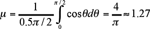
where gn is the conductance at noon, and µ is a coefficient for adjusting nonlinear change of g with time. It can be calculated from
 (8)
(8) |
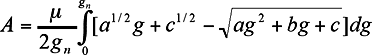
Finally, equation (7) is solved analytically:
where d=(agn2 + bgn+c)1/2. It is noted that (1) no additional parameters are introduced in this daily model, all the constants are determined by the leaf biochemical parameters in the original Farquhar model (see Table 1); (2) although equation (9) appears to be complex, it is numerically stable, and no numerical problems have been encountered in its use over large areas and under extreme conditions; (3) the analytical integration given by equation (9) is computationally efficient and avoids a daily loop using a numerical integration method.
Table 1 Procedure to Calculate Parameters in the Farquhar Model
| Step | Equation | Reference |
|---|---|---|
|
|
Kc (Michaelis-Menton constant for
CO2) and
Ko (Michaelis-Menton constant for O2) Kc = 30 x 2.1(T-25)/10 Ko = 30,000 x 1.2(T-25)/10 |
Collatz et. al. [1991] |
|
|
K (function of enzyme kinetics)
K = Kc(1+O2/Ko) |
Farquhar et al. [1980] |
|
|
Collatz et al. [1991]
Sellers et al. [1992] |
|
|
|
Vm (the maximum carboxylation rate)
f(T) = 1/(1+exp((-220,000+710(T+273))/(Rgas(T+273)))) f(N) = N/Nm Vm = Vm25 2.4(T-25)/10f(T)f(N) |
Bonan [1995] |
|
|
J (electron transport rate)
Jmax = 29.1+1.64Vm
|
Wullschleger [1993]
Farquhar and Caemmerer [1982] |
|
|
Rd (daytime leaf dark respiration)
Rd = 0.015Vm |
Collatz et al. [1991] |
For the spatial integration from leaf to canopy, a method for stratifying a canopy into sunlit and shaded leaf components has been used to upscale Farquhar's model. This is a preferable approach because the largest difference in leaf illumination in a canopy exists between sunlit and shaded leaves. The daily integration of Ac and Aj can then be made separately for each component. The calculation of sunlit leaf area and shaded leaf area is based on Norman [1982], with some modifications. One of the important modifications is the consideration of forest clumping index (see Table 2 in detail).
Table 2. Procedure to Calculate Leaf Area Index and Irradiance for Sunlit and Shade Leaves
| Step | Equation | Reference |
|---|---|---|
|
|
|
Oke [1990] |
|
|
LAIsun (sunlit leaf area index) and
LAIshade (shaded leaf area index)
LAIsun = 2 cos LAIshade = LAI -LAIsun |
Norman [1982]
Chen et al. [1999a] |
|
|
Sdir (direct solar irradiance) and
Sdif (diffuse solar irradiance)
R = Sg/(So
cos Sdir = Sg-Sdif |
Erbs et al. [1982]
Black et al. [1991] |
|
|
C (irradiance from multiple scattering of direct
radiation)
cos Sdif,under =
Sdif exp(-0.5 C = 0.07( Sdir(1.1-0.1LAI)exp(-cos |
Norman [1982]
Chen et al. [1999a] |
|
|
Ssun (sunlit-leaf irradiance) and
Sshade (shaded leaf irradiance)
Sshade = (Sdif
-Sdif, under)/LAI + C
|
Norman [1982]
Chen et al. [1999a] |
The stomatal conductance at noon can be estimated by a species-dependent maximum, which is reduced by the departure of environmental conditions from the optimum. The reduction is described by a set of environmental functions, including photosynthetic photon flux density (PPFD), temperature (T), vapor pressure deficit (VPD), and leaf water potential (LWP); that is,
| gs= gs,max f(PPFD) f(T) f(VPD) f(LWP) (10) |
Autotrophic respiration (Ra) is separated into maintenance respiration (Rm) and growth respiration (Rg) [Running and Coughlan, 1988]:
where i defines a plant component (1 for leaf, 2 for stem, and 3 for root). Maintenance respiration is temperature-dependent:
| Rm,i= Mirm,iQ10(T-Tb/10) (12) |
where Mi is biomass (sapwood for stems) of a plant component i; rm,i is maintenance respiration coefficient for component i, or respiration rate at base temperature; Q10 is the temperature sensitivity factor, and Tb is the base temperature. Growth respiration is generally considered to be independent of temperature and is proportional to GPP:
| Rg,i= rg,ira,iGPP (13) |
where rg,i is a growth respiration coefficient for plant
component i, and ra,i is carbon allocation fraction for plant
component i.
In this study, Q10 and Tb
are set to 2.3 and 20°C, respectively. Biomass and respiration coefficients
for forest covers are determined on the basis of earlier BOREAS studies
and listed in Liu et al [1999]. The carbon allocation fraction is the same
as in Forest-BGC for leaf, stem, and root [Running and Running, 1988].
The temporal and spatial scaling method
on the Farquhar's model was tested by using the tower flux measurement
data. See Chen et al.,[1999a] and Liu et al. [1999] for detail.
Notation
| A | net photosynthesis rate, µmol m-2 s-1 |
| Ac | Rubisco-limited net photosynthesis rate, µmol m-2 s-1 |
| Aj | light limited net photosynthesis rate, µmol m-2 s-1 |
| C | irradiance from multiple scattering of direct radiation, W m-2 |
| Ci | intercellular CO2 concentration , Pa |
| Ca | CO2 concentration in the atmosphere , Pa |
| D | day of year |
| g | total conductance to CO2 from cell to air, µmol m-2 s1 Pa-1 |
| gn | conductance at noon, µmol m-2 s1 Pa-1 |
| gs | stomatal conductance to CO2, m s-1 |
| gs,max | maximum stomatal conductance to CO2, m s-1 |
| J | electron transport rate, µmol m-2 s-1 |
| Jmax | light saturated rate of electron transport, µmol m-2 s-1 |
| K | function of enzyme kinetics, Pa |
| LAI | leaf area index |
| LAIsun | sunlit leaf area index |
| LAIshade | shaded leaf area index |
| O2 | intercellular O2 concentration (=21,000), Pa |
| PPFD | photosynthetically active flux density, µmol m-2 s-1 |
| Mi | biomass (or sapwood for stems) of a plant component i, kg C m-2 |
| N | foliage nitrogen concentration, % |
| Nm | maximum foliage nitrogen concentration, % |
| P | atmospheric pressure (=100,000), Pa |
| Ra | autotropic respiration, g C m-2 d-1 |
| Rd | daytime leaf dark respiration, µmol m-2 s-1 |
| Rgas | molar gas constant (= 8.3143), m3 Pa mol-1 K-1 |
| Rm | plant maintenance respiration, g C m-2 d-1 |
| Rg | plant growth respiration, g C m-2 d-1 |
| ra,i | carbon allocation fraction for plant component i |
| rm,i | maintenance respiration coefficient for plant component i, kg C kg-1 d-1 |
| rg,i | growth respiration coefficient for plant component i |
| Sdir | direct solar irradiance, W m-2 |
| Sdif | diffuse solar irradiance, W m-2 |
| Sdif,under | diffuse solar irradiance under plant canopy, W m-2 |
| Sg | global solar irradiance, W m-2 |
| So | solar constant (=1360), W m-2 |
| Ssun | sunlit-leaf irradiance, W m-2 |
| Sshade | shaded leaf irradiance, W m-2 |
| T | air temperature, °C. |
| Vm | maximum carboxylation rate, µmol m-2 s-1 |
| Vm25 | maximum carboxylation rate at 25°C, µmol m-2 s-1 |
| Wc | Rubisco-limited gross photosynthesis rate, µmol m-2 s-1 |
| Wj | light-limited gross photosynthesis rate, µmol m-2 s-1 |
| mean leaf-Sun angle (=60º for a canopy with spherical leaf angle distribution) | |
| CO2 compensation point in the absence of dark respiration, Pa | |
| solar zenith angle, degrees | |
| solar zenith angle at noon, degrees | |
| representative zenith angle for diffuse radiation transmission, degrees | |
| latitude of a location, degrees | |
| foliage-clumping index |
4. Equipment
4.1.1 Collection Environment
See AVHRR data set document in Section 1.6.4.1.2 Source/Platform
See AVHRR data set document in Section 1.6.4.1.3 Source/Platform Mission Objectives
See AVHRR data set document in Section 1.6.4.1.4 Key Variables
NDVI, SR, LAI, and land cover.4.1.5 Principles of Operation
See AVHRR data set document in Section 1.6.4.1.6 Sensor/Instrument Measurement Geometry
See AVHRR data set document in Section 1.6.4.1.7 Manufacturer of Sensor/Instrument
See AVHRR data set document in Section 1.6.
4.2 Calibration
4.2.1 Specifications
See AVHRR data set document in Section 1.6.4.2.1.1 Tolerance
See AVHRR data set document in Section 1.6.
4.2.2 Frequency of Calibration
See AVHRR data set document in Section 1.6.4.2.3 Other Calibration Information
See AVHRR data set document in Section 1.6.
5. Data Acquisition Methods
6. Observations
None.
6.2 Field Notes
None.
7. Data Description
7.1.1 Spatial Coverage
The NPP image contains 1,200 pixels in each of the 1,200 lines and cover the entire 1,000-km x 1,000-km BOREAS region. This includes the Northern Study Area (NSA), the Southern Study Area (SSA) and the transect between the SSA and NSA.
The North American Datum of 1983 (NAD83) corner coordinates and the image coordinates for the study region and the study areas are listed in Table 3.Table 3. Coordinates of Study Area, Study Region, and NPP Image
Degrees Image Coordinates Scope Corner Longitude Latitude Pixel Line Image NW -115.412 59.362 0 0 NE -93.286 61.01 1200 0 SE -93.739 50.027 0 1200 SW -110.254 48.83 1200 1200 Study region NW -111 59.979 251 4 NE -93.502 58.844 1194 235 SE -96.97 50.089 970 1192 SW -111 51 7 954 Northern study area (NSA) NW -98.82 56.247 879 511 NE -97.24 56.081 974 534 SE -97.49 55.377 955 610 SW -99.05 55.54 860 587 Southern study area (SSA) NW -106.23 54.319 396 665 NE -104.24 54.223 520 696 SE -104.37 53.419 499 782 SW -106.32 53.513 374 751 7.1.2 Spatial Coverage Map
Not available.7.1.3 Spatial Resolution
The size for all pixels is 1 km.7.1.4 Projection
The coordinate system is the Lambert Conformal Conic (LCC), with the two standard parallels at 49°N and 77°N, respectively, and the meridian at 95°W.7.1.5 Grid Description
The NPP image is projected into the LCC projection at a space of 1.0 km per pixel (grid cell) in both the X and Y directions.
7.2 Temporal Characteristics
7.2.1 Temporal Coverage
NPP in this data set represent annual values. The model is run at daily time-step. Output for given period(s) can be obtained by setting up some parameters in the model.7.2.2 Temporal Coverage Map
Not available.7.2.3 Temporal Resolution
The model is run at daily time-step. Output for given period(s) can be obtained by setting up some parameters in the model. NPP in this data set represent annual values.
7.3 Input Data Characteristics
7.3.1 Parameter/Variable
To execute BEPS over the BOREAS region, spatially explicit input data were required. These include land cover, leaf area index, available soil water holding capacity and daily meteorological (radiation, temperature, humidity, and precipitation) data.7.3.2 Variable Description/Definition
7.3.2.1 Land Cover
The land cover map of the BOREAS region is part of a 1995 Canada-wide map prepared using data from the AVHRR sensor onboard the NOAA-14 satellite. Prior to the classification, a series of data correction procedures were applied to correct atmospheric and bidirectional reflectance effects, remove contaminated pixels, and determine the growing season length [Cihlar et al., 1997a]. The average growing-season values in AVHRR channel 1 (C1, red), channel 2 (C2, near infrared) and the normalized difference vegetation index (NDVIm) were then used in the classification process. A combined enhancement-unsupervised classification methodology was used [Beaubien et al., 1999; Cihlar and Beaubien, 1998]. The resulting spectral clusters were labeled with the use of Landsat Thematic apper (TM) images and field observations. Accuracy was evaluated by provincial forest inventory agencies and in comparison with Landsat TM classifications. Land cover patterns in the AVHRR-derived map were found to be consistent with provincial maps, after allowing for scale differences. Numerical accuracy is variable, mainly because of the mixed land cover within AVHRR pixels [Cihlar et al., 1996]. Based on a digital comparison with Landsat Thematic apper classification [Klita et al., 1998], the per-class accuracy varied between 21.8% and 97.9%.7.3.2.2 Leaf Area Index (LAI)
LAI images in 1994 for the BOREAS region were derived from the same AVHRR sensor using 10-day cloud-free composite images [Cihlar et al., 1997b]. For the calculation of LAI, the NDVI was first transformed into the simple ratio (SR). Land cover specific linear SR-LAI relationships were then used to convert SR to LAI. The use of SR reduces the problem of signal saturation at high LAI values. Because the LAI of boreal vegetation is generally low and the foliage clumping reduces the effective LAI, no saturation was found for boreal forests when SR was used [Chen and Cihlar, 1996]. The algorithm for boreal conifer forests was developed by Chen and Cihlar [1996]. The algorithm for deciduous forests is based on Chen et al. [1999b], but is less accurate because of insufficient field data for the seasonal coverage and variable understory. Mixed forest was treated as an intermediate case between coniferous and deciduous forests. An algorithm for the cropland was formulated using published relationships and validated using 1996 ground measurements in 14 agricultural fields in Saskatchewan. The grassland was treated as cropland because of lack of independent measurements. To consider the effect of the seasonal greenness change in the background (understory, moss and soil/litter) of coniferous stands, a seasonal background SR trajectory was derived from AVHRR SR time series to ensure that the seasonal variation in the conifer overstory LAI was equal to or less than 25%. The formulae for the various land cover types areDeciduous forest LAI = 0.475 (SR - 2.781) Coniferous forest LAI = 1.188 (SR - Bc) ixed forest LAI = 0.592 (SR - Bm) Crop land and other land cover types LAI = 0.325 (SR - 1.5)where SR is the simple ratio; Bc and Bm are background SR trajectory for coniferous forest and mixed forest. They are calculated from Bc= 0.1(1.2x10⁻¹⁰D5 - 1.1x10⁻⁷D4 + 4.1x10⁻⁵D3 - 6.8x10⁻³D2 + 5.4x10⁻¹D - 15), and Bm= (Bc+2.781)/2, where D is the day of year. The error in a single LAI value is estimated to be ±25%.The AVHRR data temporal coverage was as follows, for 1994:
  Period   Julian Day     Season
---------  ----------     ------
Apr 11-20   101-110       Spring
Apr 21-30   111-120         ,,
ay 01-10   121-130         ,,
ay 11-20   131-140         ,,
ay 21-31   141-151         ,,
Jun 01-10   152-161       Summer
Jun 11-20   162-171         ,,
Jun 21-30   172-181         ,,
Jul 01-10   182-191         ,,
Jul 11-20   192-201         ,,
Jul 21-31   202-212         ,,
Aug 01-10   213-222         ,,
Aug 11-20   223-232         ,,
Aug 21-31   233-243         ,,
Sep 01-10   244-253       Fall
7.3.2.3 Available Water-Holding Capacity (AWC)
Soil AWC data were acquired from the Soil Landscapes of Canada (SLC) database [Shields et al., 1991]. In SLC, the land is divided into landscape polygons within which the soils are characterised by a set of attributes. The available water holding capacity (AWC) in the upper 120 cm of soil is one of the attributes contained in SLC version 1.0. About 10% of the BOREAS region was missing data (mostly in the north) in SLC version 1.0. In order to fill in the data gaps, soil texture data in SLC version 2.0 were processed, and the dominant soil texture in each polygon was determined. AWC was then assessed according to its relationship with soil texture [De Jong et al., 1984]. The AWC data in different polygons and coverages were combined, rasterized, and resampled to the same LCC projection and spatial resolution as the land cover and LAI maps. There were five levels of AWC ranging from 5 cm to 25 cm in 5 cm increments.7.3.2.4 Meteorological Data
The meteorological data were generated by the National Meteorological Center (NMC) of the National Center for Atmospheric Research (NCAR) from a medium range forecast model and provided with a grid size of about 0.9°. All meteorological data were bilinearly interpolated to each pixel at 1 km resolution after determining the geographical location of the pixel in the LCC projection.
7.3.4 Input Data Source and Format#CCRS, Canada Centre for Remote Sensing, Natural Resources Canada; CFS, Canadian Forest Service, Natural Resources Canada; CLBRR, Centre for Land and Biological Resources Research, Agriculture and Agri-Food Canada; NCAR, National Center for Atmospheric Research, Boulder, Colorado.
Parameter Source Agency# Data Type Grid System Temporal Interval Grid Size LAI AVHRR* CCRS Raster pixel/line 10 days 1 km Land cover AVHRR* CCRS & CFS Raster pixel/line Annual 1 km AWC SLC@ CLBRR Vector long term Radiation
Temperature
Humidity
PrecipitationNMC medium range forecast model NCAR Raster Gaussian daily ~0.9°
(varied with lat/long)
*Advanced very high resolution radiometer.
@Soil Landscapes of Canada.7.3.5 Input Data Range
Parameter Unit Range Growing Season Mean LAI - 0-6 Land Cover - N/A AWC m 0-0.25 Daily Mean Radiation MJ m d-1 9.0-11.0 Daily Mean Temperature °C -7.5-4.5 Daily Mean Vapour Density g m-3 4.1-7.4 Annual Total Precipitation mm y-1 180-480
7.4 Output Data Characteristics
The NPP map is in binary format, two bytes
per pixel. Values (grey levels) range from 0-32767.
8. Data Organization
Annual total NPP is contained in a separate file for the entire set of image.
8.2 Data Format(s)
NPP format: binary file, 2 byte for 1 pixel
NPP unit:   g Carbon m-2 yr-1
NPP value:  If Grey Level=0, NPP=0 (water pixel)
            If Grey Level=1, NPP=0.01 (very small)
            If Grey Level>1, NPP=Grey Level-1
9. Data Manipulations
See Section 3.
9.1.1 Derivation Techniques and Algorithms
See Section 3.
9.2 Data Processing Sequence
9.2.1 Processing Steps
BEPS is driven by land cover, leaf area index, meteorological and soil data. The temporal interval is daily for meteorological data, 10-day for LAI, annual for land cover, and long term for available water holding capacity (AWC). BEPS integrates the input data and produces output of NPP and other carbon and water cycle components. The computation is made pixel by pixel in daily time steps.9.2.2 Processing Changes
As the model is modified for a better description of ecosystems, and as more accurate spatial data become available, simulated NPP values will be more realistic. The improved can be made available when completed. See section 13.
9.3 Calculations
9.3.1 Special Corrections/Adjustments
None.9.3.2 Calculated Variables
See Section 3.
9.4 Graphs and Plots
None.
10. Errors
Sources of errors include within-pixel heterogeneity, simplification of natural processes with a daily photosynthesis model, errors in input data (land cover, LAI, meteorological and soil data), assignment of biological parameters for the various cover types, and the accuracy of image registration and processing (resampling, radiance-to-reflectance conversion, etc).
10.2 Quality Assessment
10.2.1 Data Validation by Source
Not available.10.2.2 Confidence Level/Accuracy Judgment
Because of the additive effects of sources of errors, the NPP values for individual pixels can be as large as 25-50%. However, since the model parameters and the final NPP results have been carefully calibrated using tower flux data, the major bias errors are much reduced and therefore the errors in the regional NPP estimates are expected to be smaller than 25%. The daily NPP model with sunlit and shaded leaf separation has been validated using simultaneous CO2 flux measurements made above and below forest stands [Chen et al., 1999a] and map validation was also made (see Section 10.2.3).10.2.3 Modeling Error for Parameters
In comparing modeled NPP with ground data at six forest sites [Ryan et al. 1997], close agreement is found (r=0.88, and p<0.05). The mean difference between the two data sets is 10%, with a maximum of 28% at the old jack pine in the northern study area. The root-mean-square error of modeled NPP is 34 g C /m2/yr, 12% of mean NPP in ground data set.10.2.4 Additional Quality Assessments
See Liu et al. [1999].10.2.5 Data Verification by Data Center
The data center has viewed the imagery to verify file size, format, and data range.
11. Notes
The NPP data is for 1994, a relatively normal year.
11.2 Known Problems with the Data
None.
11.3 Usage Guidance
Before uncompressing the Zip files on
CD-ROM, be sure that you have enough disk space to hold the uncompressed
data files. Then use the appropriate decompression program provided on
the CD-ROM for your specific system.
11.4 Other Relevant Information
We emphasize that the NPP results for
forests represent tree canopy only. The background (understory and moss)
contribution is not included since LAI for forest stands only includes
the overstory LAI. The LAI algorithm development only considers the overstory
LAI. Another important aspect of our calculation is the consideration of
the foliage clumping effect. We use cover type specific clumping indices
[Liu et al., 1997]. The clumping reduces sunlit leaves and increases shaded
leaves, and the NPP results calculated using the sunlit/shaded leaf model
are sensitive to the clumping index. Therefore, in any attempt to compare
the results with other model results, this should be considered. For the
users' reference, a ground study on understory contribution to total NPP
at several BOREAS sites is cited here [Ryan et al., 1997].
| Study Area | Species | NPPtotal
(g C m-2 yr-1) |
NPPunderstory
(g C m-2 yr-1) |
NPPunderstory/ NPPtotal
(%) |
|---|---|---|---|---|
| NSA | Old Black Spruce |
|
|
|
| NSA | Old Jack Pine |
|
|
|
| NSA | Old Aspen |
|
|
|
| SSA | Old Black Spruce |
|
|
|
| SSA | Old Jack Pine |
|
|
|
| SSA | Old Aspen |
|
|
|
12. Application of the Data Set
13. Future Modifications and Plans
- Consideration of sub-pixel heterogeneity by using high resolution remote sensing data. Chen [1999] showed that the largest errors of this type result from mixed water and land pixels. Using sub-pixel water area fraction can make a large improvement.
- Improving the biomass data quality. We expect that the NPP spatial distribution pattern would be more accurate if a biomass map was used rather than assigning the value by cover type. The feasibility of estimating biomass distribution from active microwave images has been demonstrated [Moghaddam et al., 1994]. Optical measurements can also be useful for this purpose for sparse canopies [Hall et al., 1995].
- Reducing the computation time step. Although the problem associated with diurnal variability is much smaller when using the integrated daily NPP model, errors are still inevitable in the daily step calculations which cannot capture sub-daily extreme events [Chen et al., 1999a]. With the improvement in computational capacity, it will soon be feasible to compute a moderate-resolution NPP distribution at much smaller time steps (minutes to hours). Such work is only possible in conjunction with a global circulation model to avoid data limitation.
14. Software
The model BEPS version 1999 is written in C and runs on a PC. The code can be easily transferred for usage in a UNIX environment. No machine-specific commands are used. Input data are in binary format. Output data are in binary format for an area and in text format for a pixel.
14.2 Software Access
The source code can be provided by contacting
Jane Liu (see section 2.1).
15. Data Access
These BOREAS data are available from the Earth Observing System Data and Information System (EOS-DIS) Oak Ridge National Laboratory (ORNL) Distributed Active Archive Center (DAAC). The BOREAS contact at ORNL is:
ORNL DAAC User Services
Oak Ridge National Laboratory
(865) 241-3952
ornldaac@ornl.gov
ornl@eos.nasa.gov
15.2 Procedures for Obtaining Data
BOREAS data may be obtained through
the ORNL DAAC World Wide Web site at http://www.daac.ornl.gov/
[Internet Link] or users may place requests for data by telephone
or electronic mail.
15.3 Output Products and Availability
Requested data can be provided electronically
on the ORNL DAAC's anonymous FTP site or on various media including, CD-ROMs,
8-MM tapes, or diskettes.
16. Output Products and Availability
The NPP image over the BOREAS region can be made available on 8-mm media or on a CD-ROM.
16.2 Film Products
None.
16.3 Other Products
These data are available on the BOREAS
CD-ROM series.
17. References
Cihlar, J. and F. Huang. 1993. User guide for the 1993 GEOCOMP products. NBIOME Internal Report, Canada Centre for Remote Sensing, Ottawa, Ontario. 9 p.
Cihlar, J. and J. Howarth. 1994. Detection and removal of cloud contamination from AVHRR composite images. IEEE Transactions on Geoscience and Remote Sensing 32: 427-437.
Cihlar, J. 1996. Identification of contaminated pixels in AVHRR composite images for studies of land biosphere. Remote Sensing of Environment 56: 149-163.
Cihlar, J., H. Ly, Z. Li, J. Chen, H. Pokrant, and F. Huang. 1997. Multitemporal, multichannel data sets for land biosphere studies: artifacts and corrections. Remote Sensing of Environment 60: 35-57.
Cihlar, J., J. Chen, and Z. Li, 1997. Seasonal AVHRR multichannel data
sets and products for studies of surface-atmosphere interactions. Journal
of Geophysical Research, 102 (D24): 29,625-29,640.
17.2 Journal Articles and Study Reports
Amiro, B. D., J. M. Chen, and J. Liu, 2000. Net primary productivity
following forest fire for Canadian ecoregions. Canadian Journal of Forest
Research, 30:939-947.
Beaubien, J., J. Cihlar, G. Simard, and R. Latifovic, 1999. Land cover from multiple Thematic Mapper scenes using a new enhancement - classification methodology, Journal of Geophysical Research, 104(D22): 27,909-27,920.
Black, T.A., J. M. Chen, X. Lee, and R. M. Sagar, 1991. Characteristics of shortwave and longwave irradiances under a Douglas-fir forest stand, Canadian Journal for Forest Research, 12: 1020-1028.
Bonan, G.B., 1995. Land-atmosphere CO2 exchange simulated by a land surface process model coupled to an atmospheric general circulation model, Journal of Geophysical Research, 100: 2817-2831.
Chen, J. M., 1999. Spatial scaling of a remotely sensed surface parameter by contexture, Remote Sensing of Environment, 69: 30-24.
Chen, J. M., and J. Cihlar, 1996. Retrieving leaf area index of boreal conifer forests using Landsat TM images, Remote Sensing of Environment, 55: 153-162.
Chen, J. M., J. Liu, J. Cihlar, and M. L. Goulden, 1999a. Daily canopy photosynthesis model through temporal and spatial scaling for remote sensing applications, Ecological Modelling, 124: 99-119.
Chen, J. M., S. G. Leblanc, J. R. Miller, J. Freemantle, S. E. Loechel, C. L. Walthall, K. A. Innanen, and H. P. White, 1999b. Compact airborne spectrographic imager (CASI) used for mapping biophysical parameters of boreal forests, Journal of Geophysical Research, 104(D22): 27,945-27,958.
Chen, J. M., W. Chen, J. Liu, and J, Cihlar, 2000. Carbon budget of boreal forests estimated from the changes in disturbances, climate, nitrogen and CO2: results for Canada in 1895-1996. Global Biogeochemical Cycle , 14: 839-850.
Chen, W. J., J. M. Chen, J. Liu, and J. Cihlar, 2000. Approaches for reducing uncertainties in regional forest carbon balance, Global Biogeochemical Cycle, 14:827-838.
Cihlar, J., 1996. Identification of contaminated pixels in AVHRR composite images for studies of land biosphere, Remote Sensing of Environment, 56: 149-163.
Cihlar, J., H. Ly, and Q. Xiao, 1996. Land cover classification with AVHRR multichannel composites in northern environments, Remote Sensing of Environment, 58: 36-51.
Cihlar, J., J. Beaubien, Q. Xiao, J. Chen, and Z. Li, 1997a. Land cover of the BOREAS region form AVHRR and Landsat data, Canadian Journal of Remote Sensing, 23: 164-175.
Cihlar, J., H. Ly, Z. Li, J. M. Chen, H. Pokrant, and F. Huang, 1997b. ultitemporal, multichannel AVHRR data sets for land biosphere studies: Artifacts and corrections, Remote Sensing of Environment, 60: 35-57.
Cihlar, J., and J. Beaubien, 1998. Land Cover of Canada 1995 Version 1.1, Digital data set documentation, Natural Resources Canada, Ottawa, Ontario.
Collatz, G. J., J. T. Ball, C. Crivet, and J. A. Berry, 1991. Physiological and environmental regulation of stomatal conductance, photosynthesis and transpiration: A model that includes a laminar boundary layer, Agricultural and Forest Meteorology, 54: 107-136.
De Jong, R., J. A. Shields, and W. K. Sly, 1984. Estimated soil water reserves applicable to a wheat-fallow rotation for generalized soil areas mapped in southern Saskatchewan, Canadian Journal of Soil Science, 64: 667-680.
Erbs, D. G., S. A. Klein, and J. A. Duffie, 1982. Estimation of diffuse radiation fraction for hourly, daily and monthly-average global radiation, Solar Energy, 28: 293-304.
Farquhar, G.D., S. von Caemmerer, and J.A. Berry, 1980. A biochemical model of photosynthetic CO2 assimilation in leaves of C3 species, Planta, 149: 78-90.
Farquhar, G.D., and S. von Caemmerer, 1982. Modelling of photosynthetic response to environmental conditions, in Encyclopedia of Plant Physiology, new series, vol. 12B, Physiological Plant Ecology II, edited by O. L. Lange, P. S. Nobel, C. B. Osmond, and H. Ziegler, pp. 549-587, Springer-Verlag, New York.
Hall, F. G. 1999. Introduction to special section: BOREAS in 1999: Experiment and science overview. Journal of Geophysical Research, 104 (D22): 27,627-27,640.
Hall, F. G., Y. E. Shimabukuro, and K. F. Huemmrich, 1995. Remote sensing of forest biophysical structure using mixture decomposition and geometric reflectance models, Ecological Applications, 5: 993-1013.
Klita, D.L., R. J. Hall, J. Cihlar, J. Beaubien, K. Dutchak, R. Nesby, J. Drieman, R. Usher, and T. Perrott, 1998. A comparison between two satellite-based land cover classification programs for a boreal forest region in northwest Alberta, Canada, in paper presented at the 20th Canadian Symposium on Remote Sensing, CRSS and ERIM International, Inc. May 1998.
Liu J., J.M. Chen, Cihlar J., and W.M. Park, 1997. A process-based boreal ecosystem productivity simulator using remote sensing inputs. Remote Sensing of Environment, 62: 158-175.
Liu J., J. M. Chen, J. Cihlar, and W. Chen, 1999. Net primary productivity distribution in the BOREAS region from a process model using satellite and surface data. Journal of Geophysical Research, 104 (D22): 27,735-27,754.
Liu J., J. M. Chen, and J. Cihlar. 2000, "Process-Modeled Net Primary Productivity over the BOREAS Region." In Collected Data of The Boreal Ecosystem-Atmosphere Study. Eds. J. Newcomer, D. Landis, S. Conrad, S. Curd, K. Huemmrich, D. Knapp, A. Morrell, J. Nickeson, A. Papagno, D. Rinker, R. Strub, T. Twine, F. Hall, and P. Sellers. CD-ROM. NASA, 2000.
Moghaddam, M., S. Durden, and H. Zebker, 1994. Radar measurement of forested areas during OTTER. Remote Sensing of Environment, 47: 154-166.
Norman, J. M. 1982. Simulation of microclimates, in Biometeorology in integrated pest management, edited by J. L. Hatfield and I. J. Thomason, p. 65-99, Academic, New York.
Oke, T. R., 1990 Boundary Layer Climates, 2nd ed., Routledge, New York.
Prince, S. D., and S. N. Goward,1995, Global primary production: A remote sensing approach, Journal of Biogeography, 22: 815-835.
Ryan, M., M. B. Lavigne, and S. T. Gower, 1997. Annual carbon cost of autotrophic respiration in boreal forest ecosystems in relation to species and climate. Journal of Geophysical Research, 102: 28,871-28,883.
Running, S. W., and J. C. Coughlan, 1988. A general model of forest ecosystem processes for regional applications, I, Hydrological balance, canopy gas exchange and primary production processes, Ecological Modelling, 42: 125-154.
Sellers, P., F. Hall, H. Margolis, B. Kelly, D. Baldocchi, G. den Hartog, J. Cihlar, M.G. Ryan, B. Goodison, P. Crill, K.J. Ranson, D. Lettenmaier, and D.E. Wickland. 1995. The boreal ecosystem-atmosphere study (BOREAS): an overview and early results from the 1994 field year. Bulletin of the American Meteorological Society. 76:1549-1577.
Sellers, P.J., F.G. Hall, R.D. Kelly, A. Black, D. Baldocchi, J. Berry, . Ryan, K.J. Ranson, P.M. Crill, D.P. Lettenmaier, H. Margolis, J. Cihlar, J. Newcomer, D. Fitzjarrald, P.G. Jarvis, S.T. Gower, D. Halliwell, D. Williams, B. Goodison, D.E. Wickland, and F.E. Guertin. 1997. BOREAS in 1997: Experiment Overview, Scientific Results and Future Directions. Journal of Geophysical Research 102(D24): 28,731-28,770.
Sellers, P. J., J. A. Berry, G. J. Collatz, C. B. Field, and F. G. Hall, 1992. Canopy reflectance, photosynthesis, and transpiration, III, A reanalysis using improved leaf models and a new canopy integration scheme, Remote Sensing of Environment, 42: 187-216.
Shields, J. A., C. Tarnocai, K. W. G. Valentine, and K. B. MacDonald, 1991. Soil landscapes of Canada, procedures manual and user's hand book, Agric. Can. Publ. 1868/E, Agric. Can., Ottawa, Ontario.
Wullschleger, S. D., 1993. Biochemical limitations to carbon assimilation
in C3 plants - A retrospective analysis of the A/Ci curves from 109 species,
Journal of Experimental Botany, 44: 907-920.
17.3 Archive/DBMS Usage Documentation
None.
18. Glossary of Terms
19. List of Acronyms
    APAR    - Absorbed Photosynthetically Active Radiation
    ASCII   - American Standard Code for Information Interchange
    AVHRR   - Advanced Very High Resolution Radiometer
    AWC     - Available Water Holding Capacity
    BOREAS  - BOReal Ecosystem-Atmosphere Study
    BORIS   - BOREAS Information System
    BEPS    - Boreal Ecosystem Productivity Simulator
    CCRS    - Canada Centre for Remote Sensing
    CFS     - Canadian Forest Service
    CLBRR   - Centre for Land and Biological Resources Research, Agriculture and Agro-Food Canada
    CD-ROM  - Compact Disk-Read-Only Memory
    CPIDS   - Calibration Parameter Input Dataset
    DAAC    - Distributed Active Archive Center
    DN      - Digital Number
    EOS     - Earth Observing System
    EOSDIS  - EOS Data and Information System
    EROS    - Earth Resources Observation System
    FPAR    - Fraction of Photosynthetically Active Radiation
    GEOCOMP - Geocoding and Compositing System
    GIS     - Geographic Information System
    GPP     - Gross Primary Productivity
    GSFC    - Goddard Space Flight Center
    LAC     - Local Area Coverage (of AVHRR)
    LAI     - Leaf Area Index
    LCC     - Lambert Conformal Conic
    LUE     - Light Use Efficiency
    MRSC    - Manitoba Remote Sensing Centre
    NAD83   - North American Datum of 1983
    NASA    - National Aeronautics and Space Administration
    NCAR    - National Center for Atmospheric Research
    NBIOME  - Northern Biosphere Observation and Modeling Experiment
    NDVI    - Normalized Difference Vegetation Index
    NMC     - National Meteorological Center
    NOAA    - National Oceanic and Atmospheric Administration
    NEP     - Net Ecosystem Productivity
    NPP     - Net Primary Productivity
    NSA     - Northern Study Area
    ORNL    - Oak Ridge National Laboratory
    PANP    - Prince Albert National Park
    PAR     - Photosynthetically Active Radiation
    RMS     - Root Mean Square
    SLC     - Soil Landscape of Canada
    SR      - Simple Ratio
    SSA     - Southern Study Area
    TE      - Terrestrial Ecology
    TF      - Tower Flux
    TIROS   - Television and Infrared Observation Satellite
    URL     - Uniform Resource Locator
    VPD     - Vapor Pressure Deficit
20. Document Information
20.1 Document Revision Date
Written: 03-Mar-2000Last Updated: 10-Nov-2000 (citation revised on 30-Oct-2002)
20.2 Document Review Date(s)
BORIS Review: 05-Apr-2000Science Review:
20.3 Document ID
dsp05_npp20.4 Citation
Cite this data set as follows (citation revised on October 30, 2002):Liu, J., J. M. Chen, and J. Cihlar. 2001. BOREAS Follow-On DSP-05 Process-Model ed Net Primary Productivity. Data set. Available on-line [http://www.daac.ornl. gov] from Oak Ridge National Laboratory Distributed Active Archive Center, Oak Ridge, Tennessee, U.S.A.
20.5 Document Curator:
webmaster@daac.ornl.gov20.6 Document URL:
http://daac.ornl.gov/BOREAS/FollowOn/guides/dsp05_avhrr_npp_doc.htmlKeywords:
BEPS
Boreal ecosystem productivity simulator
Carbon flux
Ecological modeling
Gross primary productivity
Light use efficiency
Net primary productivity
NPP
Plant respiration
Primary production