Get Data
Summary
The objective of this land cover mosaic is to provide a data product that characterises the detailed land cover of a significant portion of the BOREAS Region. Seven Landsat-5 TM images have been assembled to completely cover the BOREAS Transect. Entire TM scenes were used to create this land cover map. A detailed classification scheme was employed, permitting the extraction of virtually all land cover information that can be discerned from digitally enhanced TM images. The data are provided in a binary image format file.Note that some of the data files have been compressed using Zip compression. See Section 8.2 for details.
Data Citation
Cite this data set as follows (citation revised on October 29, 2002):Beaubien, J., R. Latifovic, J. Cihlar, and G. Simard. 2001. BOREAS Follow-On DSP-01 Landsat TM Land Cover Mosaic of the BOREAS Transect. Data set. Available on-line [http://www.daac.ornl.gov] from Oak Ridge National Laboratory Distributed Active Archive Center, Oak Ridge, Tennessee, U.S.A.
Table of Contents
- Data Set Overview
- Investigator(s)
- Theory of Measurements
- Equipment
- Data Acquisition Methods
- Observations
- Data Description
- Data Organization
- Data Manipulations
- Errors
- Notes
- Application of the Data Set
- Future Modifications and Plans
- Software
- Data Access
- Output Products and Availability
- References
- Glossary of Terms
- List of Acronyms
- Document Information
1. Data Set Overview
BOREAS Follow-On DSP-01 Landsat TM Land Cover Mosaic of the BOREAS Transect
1.2 Data Set Introduction
This data set provides land cover description
for a significant portion of the BOREAS Region, by employing 7 Thematic
Mapper (TM) scenes that collectively span the BOREAS Transect between the
Southern and the Northern Study Areas (Sellers et al., 1995). The land
cover is characterised as belonging to one of 29 land cover classes (section
7.3.2).
A detailed classification scheme was
employed, permitting the extraction of virtually all land cover information
that can be discerned in digitally enhanced TM images. However, it should
be noted that this classification does not include a separate category
for wetlands. This is because wetlands in this region are generally composed
of grass and/or shrub cover that can have very similar spectral reflectance
characteristics to non-wetland shrub and grassland classes and it is extremely
difficult to discern the two with single-date imagery.
1.3 Objective/Purpose
This classification was produced for
BOREAS Follow-on investigators who needed a land cover data set with which
to compare other measurements. It is an improved version of a 6-scene mosaic
described by Beaubien et al (1999). The objective was to map land cover
at the highest level of detail possible with TM data, especially for the
forest. This was achieved by a series of pre-processing and classification
steps, so that all the land cover detail discernible in digitally enhanced
images could be retained for preparing the land cover map.
1.4 Summary of Parameters
Land cover type (refer to section 7.3.2
for a list of classes)
1.5 Discussion
The objective of this land cover map
is to provide BOREAS regional scale modellers with a product that characterises
the land cover for a significant portion of the BOREAS Region at the TM
scale. An unsupervised classification technique was used, preceded by several
pre-processing steps to facilitate the extraction of all relevant land
cover information.
1.6 Related Data Sets
BOREAS Level-3b Landsat TM Imagery: At-sensor Radiance in BSQ Format
BOREAS TE-06 Biomass and Foliage Area Data
BOREAS TE-06 Allometry Data
BOREAS TE-13 Biometry Data
BOREAS TE-20 SSA Site Characteristics Data
2. Investigators
Dr. Josef Cihlar
2.2 Title of Investigation
BOREAS Follow-on DSP-1 TM land cover
and primary productivity in the boreal forest
2.3 Contact Information
Contact 1:
Jean Beaubien
Laurentian Forestry Centre
Sainte-Foy, Quebec
(418) 648-5822
beaubien@cfl.forestry.ca
Contact 2:
Rasim Latifovic
Canada Centre for Remote Sensing
Ottawa, Ontario
(613) 947-1816 (tel)
(613) 947-1385 (fax)
rasim.latifovic@ccrs.nrcan.gc.ca
Contact 3:
Josef Cihlar
Canada Centre for Remote Sensing
Ottawa, Ontario
(613) 947-1265
(613) 947-1406 (fax)
Josef.Cihlar@geocan.emr.ca
Contact 4:
Guy Simard
Laurentian Forestry Centre
Sainte Foy, Quebec
(418) 648-5822 (tel)
simard@cfl.forestry.ca
3. Theory of Measurements
4. Equipment
The Landsat-5 Thematic Mapper (TM) sensor system records radiation in the visible, near-IR, and thermal wavelengths. See BOREAS TM documentation for additional details.
4.1.1 Collection Environment
Landsat-5 orbits the Earth at an altitude of approximately 705 kilometres.4.1.2 Source/Platform
Landsat-5 satellite.4.1.3 Source/Platform Mission Objectives
The mission of the Landsat-5 satellite is to measure reflected radiation from Earth's surface at a spatial resolution of 30 meters and to measure the temperature of Earth's surface at a spatial resolution of 120 meters.4.1.4 Key Variables
Reflected radiation Emitted radiation Temperature4.1.5 Principles of Operation
The TM is a scanning optical sensor operating in the visible and infrared wavelengths. It contains a scan mirror assembly that directly projects the reflected Earth radiation onto detectors arrayed in two focal planes.4.1.6 Sensor/Instrument Measurement Geometry
The TM depends on the forward motion of the spacecraft for the along-track scan and uses moving mirror assembly to scan in the cross-track direction (perpendicular to the spacecraft). The Instantaneous Field of View (IFOV) for each detector from bands 1-5 and band 7 is equivalent to a 30-m square when projected to the ground; band 6 (the thermal-infrared band) has an IFOV equivalent to a 120-meter square.4.1.7 Manufacturer of Sensor/Instrument
NASA Goddard Space Flight Center
Greenbelt, MD 20771Hughes Aircraft Corporation
Santa Barbara, CA
4.2 Calibration.
The absolute radiometric calibration
between bands on both sensors is maintained by using internal calibrators
that are physically located between the telescope and the detectors and
are sampled at the end of a scan.
4.2.1 Specifications
The TM sensor is sensitive to the following spectral bands:Channel Wavelength (um) Primary Use ------- --------------- ------------------------------------------ 1 0.451 - 0.521 Coastal water mapping, soil vegetation differentiation, deciduous/coniferous differentiation. 2 0.526 - 0.615 Green reflectance by healthy vegetation. 3 0.622 - 0.699 Chlorophyll absorption for plant species differentiation. 4 0.771 - 0.905 Biomass surveys, water body delineation. 5 1.564 - 1.790 Vegetation moisture measurement, Snow cloud differentiation. 6 10.450 - 12.460 Plant heat stress measurement, Other thermal mapping. 7 2.083 - 2.351 Hydrothermal mapping.
4.2.1.1 Tolerance
None given.
4.2.2 Frequency of Calibration
The absolute radiometric calibration between bands on both sensors is maintained by using internal calibrators that are physically located between the telescope and the detectors and are sampled at the end of a scan.4.2.3 Other Calibration Information
Relative within-band radiometric calibration, to reduce "striping", is provided by a scene-based procedure called histogram equalisation. The absolute accuracy and relative precision of this calibration scheme assumes that any change in the optics of the primary telescope or the "effective radiance" from the internal calibrator lamps is insignificant in comparison to the changes in detector sensitivity and electronic gain and bias with time and that the scene-dependent sampling is sufficiently precise for the required within-scan destriping from histogram equalisation. Each TM reflective band and the internal calibrator lamps were calibrated prior to launch using lamps in integrating spheres that were in turn calibrated against lamps traceable to calibrated National Bureau of Standards lamps. Sometimes the absolute radiometric calibration constants in the "short-term" and "long-term parameters" files used for ground processing have been modified after launch because of inconsistency within or between bands, changes in the inherent dynamic range of the sensors, or a desire to make quantized and calibrated values from one sensor match those from another.
5. Data Acquisition Methods
TM         Calibration gain         Characteristic   Solar irradiance
Spectral   (counts/(W/m**2/         wavelength       (W/m**2/
Band       sr/micrometre))          (micrometre)     micrometre)
--------   ---------------------    ------------     -----------
1          G=(-3.58E-05)*D+1.376    0.4863           1959.2
2          G=(-2.10E-05)*D+0.737    0.5706           1827.4
3          G=(-1.04E-05)*D+0.932    0.6607           1550.0
4          G=(-3.20E-06)*D+1.075    0.8382           1040.8
5          G=(-2.64E-05)*D+7.329    1.677             220.75
7          G=(-3.81E-04)*D+16.02    2.223              74.960
6. Observations
In general, the data quality was acceptable from the atmospheric transparency viewpoint, except for scene Path 33/Row 31 which appeared to be hazy over its SW part. Significant radiometric differences were also apparent as a result of seasonal (day of acquisition) and interannual differences, most likely due to varying precipitation regimes. These differences were dealt with at the classification and labelling stages.
6.2 Field Notes
Field observations were collected as
part of the accuracy assessment procedure (refer to section 10.2.1).
7. Data Description
7.1.1. Spatial Coverage
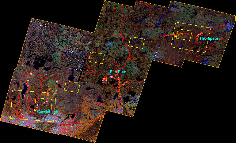
The seven images cover an area of 142854.15 km2, over 159 million pixels, 30 metres by 30 metres in size, and include both the BOREAS Southern and Northern Study Areas. Because of the orbital geometry, a small area between images Path/Row 37/21 and 35/21 was omitted when the images were selected.Corner Longitude Latitude ------------------ ---------------- ---------------- Upper Left Corner 106°46'55.71" W 56°51'25.89" N Upper Right Corner 96°06'30.92" W 56°51'25.89" N Image Centre 101°26'43.32" W 54°50'25.87" N Lower Left Corner 106°46'55.71" W 52°49'25.86" N Lower Right Corner 96°06'30.92" W 52°49'25.86" N7.1.2 Spatial Coverage Map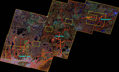
7.1.3 Spatial Resolution
Each pixel represents a 30-meter by 30-meter area on the ground.7.1.4 Projection
The projection is defined by the following parameters:Georeference Units : LONG/LAT Projection : Geographic (geodetic) Datum - Ellipsoid : WGS 1984 (Global Definition) - WGS 847.1.5 Grid Description
The data are referenced to the projection described in section 7.1.4.Pixel Size (in Degrees) : 0.00046 Lon 0.00029 Lat (Equivalent Deg,Min,Sec) : 0° 00' 01.65" 0° 00' 01.03"
7.2 Temporal Characteristics
7.2.1 Temporal Coverage
See section 7.2.2.7.2.2 Temporal Coverage Map
The data that were used to produce this classification were collected by the Landsat-5 TM on the following dates:Path Row Date and time of acquisition Scene centre ---- --- ---------------------------- ------------------------------ 33 21 June 12, 1992 16:50:20 55° 54' 46" N / 97° 59' 49" W 34 21 August 06, 1992 16:56:30 55° 54' 42" N / 99° 32' 24" W 35 21 August 11, 1991 17:06:50 55° 54' 48" N / 100° 59' 16" W 37 21 August 28, 1998 17:36:24 55° 24' 44" N / 104° 18' 19" W 35 22 August 11, 1991 17:06:50 54° 29' 37" N / 101° 43' 48" W 36 22 July 30, 1996 17:00:42 53° 46' 34" N / 103° 26' 37" W 37 22 August 09, 1991 17:14:50 53° 59' 30" N / 105° 06' 43" W7.2.3 Temporal Resolution
Each TM scene was collected at a single point in time as indicated in section 7.2.2.
7.3 Data Characteristics
7.3.1. Parameter/Variable
Land cover type.7.3.2 Variable Description/Definition
The classification scheme was designed to meet three objectives: 1) retain as much information about land cover in the Region as possible, especially regarding forest types and conditions; 2) be compatible with other classifications employed by boreal ecosystem investigators; and 3) be applicable to Landsat TM (i.e. all the necessary information to differentiate between the classes should be available in a single-scene TM image).
Class Descriptions
Two sets of pixel values are shown for each class. The number preceding the class name refers to the final classification, each class having a unique identifier. The second set of numbers (after the name) refers to spectral clusters that have been agglomerated to produce the final class; they thus provide additional (spectral) information. Note that the file "tm_mosaic_cls1" (section 8.2.1) contains the first set of pixel identifiers, and the file "tm_mosaic_cls2" contains the second set.Pixel Class Value Name ------------------ 7 - Coniferous high crown density black spruce (includes spectral clusters 6, 7) 11 - Coniferous high crown density black spruce and Jack pine (11, 12, 15, 18) 21 - Coniferous high crown density black spruce younger (21, 19, 17, 31) 22 - Coniferous medium crown density jack pine (22) 32 - Coniferous medium crown density black spruce, jack pine (33, 32, 34, 29, 10) 25 - Coniferous medium crown density black spruce (20, 25, 28) 43 - Coniferous low crown density black spruce, jack pine (43, 41) 59 - Coniferous low crown density jack pine (59, 37, 49) 55 - Coniferous very low density (55, 52, 50, 65) 79 - Deciduous high crown density (83, 79, 78, 88, 86, 93) 80 - Deciduous medium crown density (80, 75, 68, 66) 99 - Deciduous low broadleaf cover (99, 111) 39 - Mixed coniferous high density (39) 36 - Mixed coniferous medium density (36) 69 - Mixed deciduous forest (69, 73, 62) 53 - Mixed forest (53, 48) 85 - Shrubs and grassland (85, 72, 71, 126) 13 - Burn recent bare area (13) 35 - Burn recent sparse vegetation cover (35, 30, 54, 63, 47) 113 - Burn rock outcrops (51, 113, 130, 131) 81 - Older burns shrub-grass cover (81, 106, 84, 109) 64 - Old burns mixed regeneration cover (64, 77) 134 - Bare disturbed area (134, 143) 112 - Bare disturbed areas sparse vegetation cover (133, 112, 120, 123, 118, 149) 160 - Cropland high biomass (160) 161 - Cropland medium biomass (161) 162 - Cropland low biomass (162) 1 - Water (1, 2, 3, 4, 5, 9) 150 - Clouds (150, 128, 127)The class descriptions follow below. Note that the sole purpose of the numbering scheme used here is to indicate the hierarchy among the categories.
Class 1.0 Coniferous (>80% coniferous trees) Class 1.1 High crown density (>60%)
This class, especially prevalent in the Northeast portion of the mapped area, contains older black spruce (BS) forest (older than ~40 years).
This class is also dominated by old black spruce forest, like 1.1.1, but is more widely spread in the region and commonly includes jack pine (JP) trees; if desirable, 1.1.1 and 1.1.2 may be merged.
As most of this region was repetitively burned in the past, this class is particularly dispersed in the area. It may contain a small proportion of broadleaf species (<20%) and some jack pine stems; ëyoungerí refers to approximately 20-40 years.Class 1.2 Medium crown density (40-60%)
In this region, medium crown density forests are generally young (~ 20-40 years). It should be noted that the species (BS or JP) may influence the apparent density. For example, a dense (>60%) jack pine stand may be part of a medium density class because of the foliage pattern and the influence of the ground cover (particularly lichens) more easily apparent then under a dense black spruce stand.
Typically, a jack pine forest on a drier site with lichen commonly present in the understory.
Lichens may also be present, but generally has a green understory; this class is particularly widespread in the region.
Generally located on more humid sites, this class can include a small proportion of broadleaf species.Class 1.3 Low crown density (25-40%)
Commonly located on wet sites with a proportion of broadleaf vegetation (mostly shrubs); occasionally young tree canopy after older burns (> 10 years).
Lichens commonly present in the understory; occasionally this class is located in burned areas with mixed cover (dead stems, bare soil, rock outcrops); an understory with abundant lichens seems to lower the apparent density. There is confusion in this class with some dried-up wetlands.Class 1.4 Very low crown density (10-25%) (DN = 55)
Commonly located on wet sites with a proportion of broadleaf vegetation (mostly shrubs) in the southern portion of the region; in the northern areas, some regenerating cover after burns.Class 2.0 Deciduous (>80% deciduous trees) Class 2.1 High crown density (> 60%) (DN = 79)
Almost exclusively in the southern part of the area; elsewhere some rare younger, dense broadleaf cover (or high shrubs) can be in this class.Class 2.2 Medium crown density (40-60%) (DN = 80)
Mainly in the southern part of the area in the vicinity of high-density deciduous forest; transitions between high and medium densities may frequently occur locally; the density values refer mainly to the dominant broadleaf trees; some conifers may be present in lower strata. After perturbations (fires), this class may combine young and short broadleaf cover with possible conifer regeneration.Class 2.3 Low broadleaf cover (DN = 99)
Mostly in the southern part of the area, after perturbations such as previous cut-overs, burns, and cropland areas with shrub cover.Class 3.0 Mixed forest (20-80% coniferous or deciduous trees) Class 3.1 Mixed coniferous (> 60% coniferous trees)
Mainly among southern mixed forest, some patches exist in northern old burns (>10 years).
Mainly young forest cover in northern old burns.Class 3.2 Mixed deciduous forest (> 60% deciduous, density > 60%) (DN = 69)
Mainly located in the southern part of the area within high crown density deciduous forest class of high crown density.Class 3.3 Mixed forest (40-60% coniferous/deciduous, density > 60%) (DN = 53)
Among southern broadleaf and mixed forest cover, but also numerous patches of young forest cover after old burns in northern areas.Class 4.0 Open land (tree crown density <10%) Class 4.1 Shrubs and grassland (DN = 85)
Typically contains wetlands in southern areas; very few patches after more or less recent burns; some trees can be present.Class 4.2 Burns
Note that some TM scenes predate fieldwork by up to seven years; during this period, vegetation on burns has regenerated.
Dead standing stems are commonly present. Confusion exists with some patches of medium density jack pine cover class with lichen understory, class 22.
Rock outcrops with very sparse vegetation after burns.
Conifer regeneration can be present; also some patches of open land with partial green vegetation, like some wetlands.
Conifer regeneration can be present; also some patches of similar cover within wetlands.
Also mixed low cover in wetland areas.Class 4.3 Bare disturbed areas (DN = 134)
Very sparse vegetation cover, mainly located in areas recently disturbed by cut-overs in the southern portion of the area.Class 4.4 Disturbed areas, sparse vegetation cover (DN = 112)
This class with sparse vegetation cover is located mainly in areas recently disturbed by cut-overs in the southern part of the area; a few exceptions are some patches in burned areas; conifer regeneration can be present (recall the acquisition dates of the imagery).Class 5.0 Cropland
No attempt was made to differentiate crop types, because the primary interest is forest cover, and the varying acquisition dates make crop identification difficult. The categories below refer broadly to different crop types, but the phenological differences cause large confusion.Class 5.1 High biomass (DN = 160) Class 5.2 Medium biomass (DN = 161) Class 5.3 Low biomass (DN = 162) Class 6.0 Non-vegetated land Class 6.1 Water bodies (DN = 1)
This class contains some cloud shadowsClass 6.2 Clouds (DN = 150) 7.3.3 Unit of Measurement
Land Cover type - coded but unitless value.7.3.4 Data Source
Landsat-5 TM (refer to section 4.).Forest cover maps of the area were acquired to identify training fields. The following basic source maps were used:7.3.5 Data Range
- Manitoba Department of Natural Resources, Provincial Forest Inventory Maps. These maps are compiled from aerial photographs at a scale of 1:15,840. Each map covers an area of about 93 km2. Maps identify stands by number, assigned within each map; a separate legend sheet for each map provides details about each stand.
- Saskatchewan Department of Tourism and Renewable Resources, Inventory Maintenance Maps. These maps are compiled from aerial photographs at a scale of 1:12,500. Each map covers a 10x10 km area. Stand information code on the map include stand number, species age, height, and canopy information.
Pixel values of 0 to 162, stored as 8-bit integers.
7.4 Sample Data Record
Not applicable for image data.
8. Data Organisation
The smallest amount of data that can be ordered from these data is the entire data set.
8.2 Data Format
8.2.1 Uncompressed Data Files
The classification product contains two image files, each are unsigned 8 bit binary files, with a size of 23341 pixels by 14139 lines.The image files have been compressed with the MS Windows-standard Zip compression scheme. These files were compressed using Aladdin's DropZip on a Macintosh. DropZip uses the Lempel-Ziv algorithm (Welch, 1994), also used in Zip and PKZIP programs. The compressed files may be uncompressed using PKZIP (with the -expand option) on MS Windows and UNIX, or with StuffIt Expander on the Mac OS. You can get newer versions from the PKZIP Web site at http://www.pkware.com/download-software/ [Internet Link].
- tm_mosaic_cls1.img: Classified image with values from 1 to 150 with zero values (0) used as fillers for non-image (no data) areas of the image: contains a unique identifier for each final class (refer to section 7.3.2).
- tm_mosaic_cls2.img: Classified image with values from 1 to 150 with zero values (0) used as fillers for non-image (no data) areas of the image: contains a unique identifier for each spectral cluster; one or more clusters were merged to form the final classes (refer to section 7.3.2).
9. Data Manipulations
Not applicable.
9.1.1 Derivation Techniques and Algorithms9.2 Data Processing Sequence
None given.
9.2.1 Data Processing Steps9.2.2 Processing Changes
- Image selection and pre-processing
The intent was to obtain land cover classification compatible with the BOREAS experimental period (1994-1996). Given the limitations of data availability (primarily due to cloud cover), images from several years were used. For the most part, the resulting classification is representative of land cover during BOREAS because of the low rate of land cover change during the 1990's. The selected images are listed in section 7.2.2.
A new radiometric normalisation procedure was used to establish radiometric consistency among the seven TM scenes. The principle of the method is to employ overlapping sections among the scenes, assuming that there are at least some areas within these whose reflectance properties have not changed between the imaging dates (Du et al., 2000). The procedure avoids any loss of radiometric detail during the normalisation, and ensures consistency across the entire mosaic, regardless of the sequence of scenes in the mosaicking.- Image classification
A modified version of the Enhancement-Classification Method (ECM) (Beaubien et al., 1999) was used to classify the image mosaic. The ECM procedure is intended to capture most of the information visible in an enhanced image by converting the image into a classification through various generalization steps. It was designed to be as reproducible as possible for an interactive classification. The main modification to the original methodology is the use of an unsupervised classifier in step #2 below instead of image quantization. Image filtering, employed to help in the selection of the more important image mean values (signatures), was also modified. In summary, the modified ECM consists of the following phases:
- Image contrast enhancement
The purpose of the enhancement is to bring out the distinctions among various classes of interest so that they can be more easily viewed in the subsequent steps. It is carried out in three steps: viewing of the data, sampling of cover types with low and high values in each spectral band, and digital stretch.- Unsupervised classification
The purpose of this part of the process is to produce a first classification, which captures most of the information visible in the initial enhanced image. A K-Means method (Tou and Gonzales, 1974) was used to classify the stretched image into 150 clusters. After computing a pseudo colour table (PCT) for the enhanced image, the classified image closely resembles the enhanced input image.- Minimum distance re-classification
A second level of generalization is reached by a re-classification from a selection of the more significant signatures generated by the unsupervised classifier. This is carried out in three steps, first, by image filtering (mode and sieve filters) to "flatten" the image by making classes more uniform over groups of spatially adjacent pixels. The next step includes selection of all visible (thus more significant) cover types. Lastly, a minimum distance classification on the initial enhanced image according to the signatures of the selected cover types. To reduce the number of clusters before manual agglomeration, those three steps are optionally repeated. After each iteration, the classification results are carefully compared to the initial unsupervised classification, using the same pseudo-colour table. Other signatures may be added if suitable.- Cluster agglomeration and labeling
The purpose of this step is to group spectral clusters representing the same ground cover types. Since the last classified image closely resembles the original image, where image colours associated with the basic cover types are known, a substantial degree of agglomeration can be completed on the basis of colour patterns. Additional tools may include examination of the cluster mean digital value through a distance table, and spatial proximity values between clusters. For the remainder, independent knowledge of ground conditions in specific areas is required, as in other classification methods.
None.
9.3 Calculations
9.3.1 Special Corrections/Adjustments
None.9.3.2 Calculated Variables
Refer to PCI CSG and MLC programs.
9.4 Graphs and Plots
The area occupied by individual classes
is as follows:
Pixel
Number     Area [km2]       Percent
-----------------------------------
7           4551.1461       3.1859%
11         11184.5817       7.8294%
21         12431.7315       8.7024%
22          3377.6496       2.3644%
32         16748.0874      11.7239%
25         10621.206        7.4350%
43          7990.4637       5.5934%
59          5389.1595       3.7725%
55         13722.4071       9.6059%
79          3908.4408       2.7360%
80          5158.6686       3.6111%
99          1160.6319       0.8125%
39          2958.075        2.0707%
36          2026.5147       1.4186%
69          3308.2668       2.3158%
53          4043.7774       2.8307%
85          4177.5588       2.9244%
13           861.1092       0.6028%
35         10667.6442       7.4675%
113         1683.2673       1.1783%
81          5954.6016       4.1683%
64          4617.3114       3.2322%
134          363.4947       0.2545%
112         1016.1828       0.7113%
160         2315.1312       1.6206%
161          799.0407       0.5593%
162         1818.0036       1.2726%
-----------------------------------
Total     142854.15          100%
10. Errors
This classification does not include a separate category for wetlands. This is because wetlands in this region are generally composed of grass and/or shrub cover with different heights, densities, and the ratios of live-to-dead leaf biomass. Consequently, they can have very similar spectral reflectance characteristics to shrub, grassland, and some burn classes. It might be possible to use late spring images as an additional data source because surface water should have a stronger influence on the spectral reflectance. Alternatively, radar images might be helpful. However, such differentiation does not appear to be feasible with a single-date TM image taken during the growing season. Thus, most wetland cover types are in the shrub and grassland class (85), and some are contained within the burn classes (81, 64, 35). A similar situation is present in the southern part of the mosaic where grass fields in agriculture area are classified as class 81.
10.2 Quality Assessment
10.2.1 Data Validation by Source
The classification was checked qualitatively using aerial photographs, and quantitatively using field data. Three types of field sites were used:For the accuracy assessment, each site from the BOREAS auxiliary site set and the additional set was assigned to one of the 29 classes, based on a consensus of two interpreters. The corresponding class on the map was defined to be the majority class occurring in the 3x3 window centred on the site.
- BOREAS auxiliary sites 'B': these sites were carefully documented using aerial photographs, and described in the field using forest mensuration and site description methods (Halliwell and Apps, 1997). A total of 55 sites were documented in this manner.
- Additional sites: in late September and early October of 1998, a field survey was undertaken to obtain additional data for accuracy assessment. Due to access limitations and the large area to be covered, the criteria for site locations were the representativeness of the various forest classes and conditions, sufficiently large patch size (to compensate for potential geolocation uncertainties), and proximity to the existing road network. This was accomplished by pre-processing the mosaicked TM image to locate spectrally homogenous patches, overlaying the road network, and printing the result at a large scale for use in the field. The above procedure resulted in a somewhat uneven distribution of test sites, as indicated in the table below, but further improvements were not feasible with the available resources.
Two types of sites were used: 'S', sites with photographs (overstory, understory, horizontal view) and physiognomic descriptions (overstory, understory); and 'M', sites with a photograph (horizontal view) and vegetation class identification. The location of each 'S' site was established with a GPS, and each 'M' site by landmarks on the TM enhancements. A total of 94 'M' sites and 89 'S' sites were located across the region. In addition, high-resolution GPS point measurements were taken to facilitate accurate registration of the TM mosaic.10.2.2 Confidence Level
Based on the qualitative and quantitative accuracy assessments (section 10.2.1, 10.2.3), we have high confidence in the accuracy of the classification. As noted above, the main limitation is absence of a wetland class. In addition, accuracies could be lower in areas from which no field sites were located, e.g. areas farther from the existing road network.10.2.3 Measurement Error for Parameters and Variables
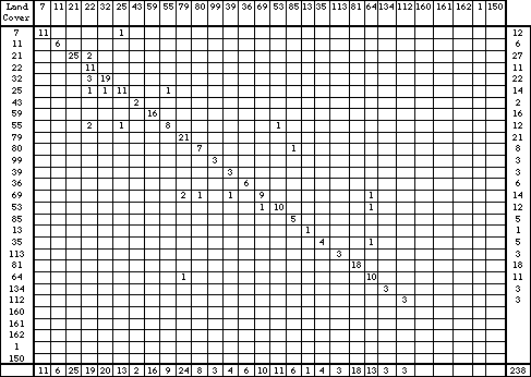
The following tables and statistics were derived in assessing the classification accuracy:A. Number of sites by category and agreement
      Class      'M' Sites | 'S' Sites | 'B' Sites | All Sites    Pct
No.   Name       No. Match | No. Match | No. Match | No. Match    Match
------------------------------------------------------------------------
7    CHD BS       6    5      3    3      3    3     12   11      0.917
11   CHD BS/JP    1    1      1    1      4    4      6    6      1.000
21   CHD BSY      7    5     14   14      6    6     27   25      0.926
22   CMD JP       5    5      4    4      2    2     11   11      1.000
32   CMD BS/JP    4    4      8    7     10    8     22   19      0.864
25   CMD BS       3    3      8    7      3    1     14   11      0.786
43   CLD BS/JP    1    1      1    1      0    0      2    2      1.000
59   CLD JP       6    6      7    7      3    3     16   16      1.000
55   CVLD         4    4      3    2      5    2     12    8      0.667
79   BHD          8    8      7    7      6    6     21   21      1.000
80   BMD          5    5      3    2      0    0      8    7      0.875
99   BLD          3    3      0    0      0    0      3    3      1.000
39   MCHD         0    0      3    3      0    0      3    3      1.000
36   MCMD         2    2      2    2      2    2      6    6      1.000
69   MB           5    3      4    2      5    4     14    9      0.643
53   MIX          2    1      6    6      4    3     12   10      0.833
85   SHR/GRASS    3    3      2    2      0    0      5    5      1.000
13   B-recent     1    1      0    0      0    0      1    1      1.000
35   B-recent     4    3      1    1      0    0      5    4      0.800
113  B-rock-out-  2    2      1    1      0    0      3    3      1.000
      crops
81   B-old       11   11      6    6      1    1     18   18      1.000
      shrub/grass
64   B-old mixed  7    6      3    3      1    1     11   10      0.909
      regeneration
134  Bare         2    2      1    1      0    0      3    3      1.000
      disturbed
112  Bare         2    2      1    1      0    0      3    3      1.000
      disturbed sparse
160  CROP/HB*
161  CROP/MB*
162  CROP/LB*
1    WATER*
150  CLOUD*
------------------------------------------------------------------------
TOTAL            94   86     89   83     55   46    238  215      0.903

* no auxiliary sites available for this class
B. Confusion matrix
The following confusion matrix shows results of the accuracy assessment. It is evident that the overall accuracy is quite high. The confusion that did occur was mostly between adjacent density classes or the proportions of coniferous and deciduous classes.Error Matrix of the Classification Map BOREAS MOSAIC V3
Summarising the classes into major groups, the classification accuracy was as follows:
Class           % Correct
-------------------------
Coniferous        90.0%
Deciduous         96.9%
Mixed             80.0%
Disturbed/other   95.9%
------------------------
Overall Correct   90.7
The overall kappa value (Congalton, 1991) was 0.8977 or 89.8% better than chance agreement.
10.2.4 Additional Quality Assessments
None.10.2.5 Data Verification by Data Center
This image was viewed to make sure that it matched the product description and appeared to be a classification image of a part of the BOREAS region.
11. Notes
The user should keep in mind that the original images were taken in different years. The class descriptions and the map accuracy should also be considered in using this product.
11.2 Known Problems with the Data
None
11.3 Usage Guidance
Users should be aware of accuracy limitations
as well as problems listed in Section 10.
11.4 Other Relevant Information
None.
12. Application of the Data Set
13. Future Modifications and Plans
14. Software
Various proprietary programs in the EASI/PACE image processing software from PCI, Inc. were used to classify the image. Zip uses the Lempel-Ziv algorithm (Welch, 1994) used in the zip and PKZIP commands.
14.2 Software Access
EASI/PACE is a proprietary software
package developed by PCI, Inc. Contact PCI for details.
PCI, Inc.Zip software is available from many Web sites across the Internet. You can get newer versions from the PKZIP Web site at http://www.pkware.com/download-software/ [Internet Link]. Versions of the decompression software for MS Windows, Mac OS, and several varieties of UNIX systems are included on the CD-ROMs.
50 West Wilmot St.
Richmond Hill
Ontario, Canada L4B 1M5
(905) 764-0614
(905) 764-9604 (fax)
15. Data Access
These BOREAS data are available from the Earth Observing System Data and Information System (EOS-DIS) Oak Ridge National Laboratory (ORNL) Distributed Active Archive Center (DAAC). The BOREAS contact at ORNL is:
ORNL DAAC User Services
Oak Ridge National Laboratory
(865) 241-3952
ornldaac@ornl.gov
ornl@eos.nasa.gov
15.2 Procedures for Obtaining Data
BOREAS data may be obtained through
the ORNL DAAC World Wide Web site at http://www.daac.ornl.gov/
[Internet
Link] or users may place requests for data by telephone or electronic
mail.
15.3 Output Products and Availability
Requested data can be provided electronically
on the ORNL DAAC's anonymous FTP site or on various media including, CD-ROMs,
8-MM tapes, or diskettes.
16. Output Products and Availability
These data can be made available on CD-ROM.
16.2 Film Products
None.
16.3 Other Products
None.
17. References
Friedel J. P., Fisher T. A. 1987. Mosaics - a system to produce state-of-the-art satellite imagery for resource managers. Geocarto International 2(3): 5-12.
PACE Image Analysis Kernel Version 5.2. 1993. PCI Inc. Richmond Hill, Ontario.
Richards, J. A. 1986. Remote Sensing Digital Image Analysis: An Introduction. Springer Verlag.
Welch, T.A. 1984, A Technique for High Performance Data Compression, IEEE Computer, Vol. 17, No. 6, pp. 8 - 19.
Du, Y., Cihlar, J., Beaubien, J., and Latifovic, R. 2000. Radiometric
normalization, compositing and quality control for satellite high resolution
image mosaics over large areas. IEEE Transactions on Geoscience and Remote
Sensing (submitted).
17.2 Journal Articles and Study Reports
Beaubien, J., J. Cihlar, G. Simard, and R. Latifovic. 1999. Land cover
from multiple Thematic Mapper scenes using a new enhancement-classification
methodology. Journal of Geophysical Research 104(D22): 27909-27920.
Congalton, R.G. 1991. A review of assessing the accuracy of classifications of remotely sensed data. Remote Sensing of Environment 37: 35-41.
Halliwell, D.H., and M. J. Apps. 1997. BOReal Ecosystem-Atmosphere Study (BOREAS biometry and auxiliary sites: locations and descriptions. Canadian Forest Service, Natural Resources Canada, Edmonton, Alberta. 120p.
Sellers, P., F. Hall, H. Margolis, B. Kelly, D. Baldocchi, G. den Hartog, J. Cihlar, M.G. Ryan, B. Goodison, P. Crill, K.J. Ranson, D. Lettenmaier, and D.E. Wickland. 1995. The boreal ecosystem-atmosphere study (BOREAS): an overview and early results from the 1994 field year. Bulletin of the American Meteorological Society. 76(9):1549-1577.
Tou, J.T., and R.C. Gonzales. 1974. Pattern recognition principles.
Addison-Wesley Publishing Co.
17.3 Archive/DBMS Usage Documentation
None.
18. Glossary of Terms
19. List of Acronyms
ASCII     - American Standard Code for Information Interchange
BOREAS    - BOReal Ecosystem-Atmosphere Study
BORIS     - BOREAS Information System
BPI       - Bytes Per Inch
CCRS      - Canadian Centre for Remote Sensing
CD-ROM    - Compact Disk-Read-Only Memory
DAAC      - Distributed Active Archive Center
EOS       - Earth Observing System
EOSAT     - Earth Observing Satellite Company
EOSDIS    - EOS Data and Information System
GMT       - Greenwich Mean Time
GPS       - Global Positioning System
IFOV      - Instantaneous Field of View
LCC       - Lambert Conformal Conic projection
MSA       - Modeling Sub-Area
MSS       - Multispectral Scanner
NAD83     - North American Datum of 1983
NASA      - National Aeronautics and Space Administration
NSA       - Northern Study Area
ORNL      - Oak Ridge National Laboratory
PANP      - Prince Albert National Park
SSA       - Southern Study Area
TE        - Terrestrial Ecology
TM        - Thematic Mapper
URL       - Uniform Resource Locator
UTM       - Universal Transverse Mercator
WGS84     - World Geodetic System of 1984
WRS       - Worldwide Reference System
WWW       - World Wide Web
20. Document Information
20.1 Document Revision Dates
Written: 06-Jul-2000Last Updated: 10-Jan-2001 (citation revised on 29-Oct-2002)
20.2 Document Review Dates
Science Review: 12-Dec-200020.3 Document ID
dsp01_tm20.4 Citation
Cite this data set as follows (citation revised on October 29, 2002):Beaubien, J., R. Latifovic, J. Cihlar, and G. Simard. 2001. BOREAS Follow-On DSP-01 Landsat TM Land Cover Mosaic of the BOREAS Transect. Data set. Available on-line [http://www.daac.ornl.gov] from Oak Ridge National Laboratory Distributed Active Archive Center, Oak Ridge, Tennessee, U.S.A.
20.5 Document Curator:
webmaster@daac.ornl.gov20.6 Document URL:
http://daac.ornl.gov/BOREAS/FollowOn/guides/dsp01_tm_landcover_doc.htmlKeywords
LAND COVER
LANDSAT TM
CLASSIFICATION