Documentation Revision Date: 2025-11-05
Dataset Version: 1
Summary
This dataset holds 257 files: 252 GeoTIFFs, four files in comma-separated values format, and one GeoPackage file.
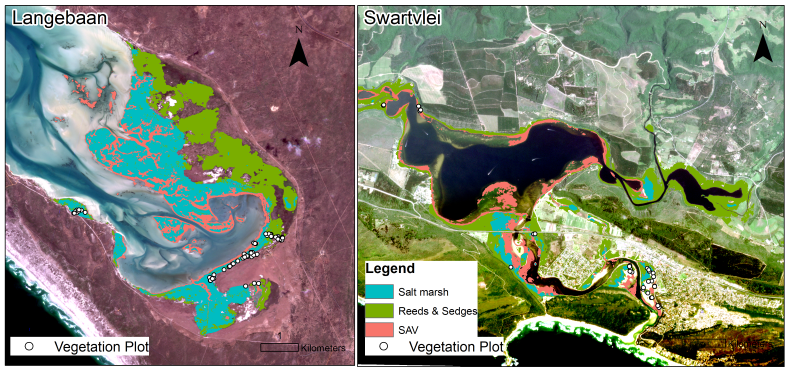
Figure 1. Locations of field plots and classified vegetation types in the Langebaan and Swartvei estuaries on the coast of South Africa. Basemap: Planetscope imagery.
Citation
Campbell, A., E. Adam, L. Fatoyinbo, D.J. Jensen, M. Simard, K. Smith, P. Thakali, A. Barrenblit, L. Naidoo, H. van Deventer, and A. Stovall. 2025. BioSCape Estuary Wetland Vegetation Plot Data and Habitat Extents, South Africa. ORNL DAAC, Oak Ridge, Tennessee, USA. https://doi.org/10.3334/ORNLDAAC/2441
Table of Contents
- Dataset Overview
- Data Characteristics
- Application and Derivation
- Quality Assessment
- Data Acquisition, Materials, and Methods
- Data Access
- References
Dataset Overview
This dataset provides vegetation information for 64 coastal wetland plots and coastal wetland extent maps for three habitat classes in 84 estuaries in South Africa. The vegetation plot data include vegetation species occurrence, percent cover, salinity, representative vegetation heights, porewater salinity, and ground temperature. In situ plot data were collected between October 27, 2023 and November 10, 2023 in Swartvlei Estuary, Wilderness Lakes, Knynsa Estuary, and Langebaan Lagoon within lands administered by the South African National Parks. The habitat extent maps were created for 84 estuaries across the Greater Cape Floristic Region. The classification is a single point in time representing the growing season when the plot data were collected (December 2023-January 2024). The habitat extent data were created with PlanetScope satellite classified with a U-Net semantic segmentation algorithm. The habitats classified are salt marsh, submerged aquatic vegetation, and reeds & sedges. Plot and habitat data were collected and created to inform analysis of the imaging spectroscopy and LiDAR data collected as part of the BioSCape field campaign. The data are provided in cloud optimized GeoTIFF, comma separated values, and geopackage formats.
Project: Biodiversity Survey of the Cape (BioSCape)
The Biodiversity Survey of the Cape (BioSCape) is an international collaboration between South Africa and the United States to study biodiversity in South Africa’s Greater Cape Floristic Region (GCFR). The GCFR was selected due to two exceptional hotspots of both terrestrial and aquatic biodiversity. The GCFR is listed among the World’s 200 Significant Ecoregions. The BioSCape is an integrated field and airborne campaign occurring in 2023. The campaign will collect UV/visible to short wavelength infrared (UVSWIR) and thermal imaging spectroscopy and laser altimetry LiDAR data over terrestrial and aquatic targets using four airborne instruments: Airborne Visible InfraRed Imaging Spectrometer - Next Generation (AVIRIS-NG), Portable Remote Imaging SpectroMeter (PRISM), Land, Vegetation, and Ice Sensor (LVIS), and Hyperspectral Thermal Emission Spectrometer (HyTES). The anticipated airborne data set is unique in its size and scope and unprecedented in its instrument combination and level of detail. These airborne data will be accompanied by a range of biodiversity-related field observations. BioSCape’s primary objective is to understand the structure, function, and composition of the region’s ecosystems, and to learn about how and why they are changing in time and space.
Related Publication
Campbell, A., Adam, E., Adams, J. B., Barrenblitt, A., Fatoyinbo, T., Jensen, D., et al. (2025). Monitoring coastal estuarine habitats for biodiversity along the temperate bioregion of South Africa. Journal of Geophysical Research: Biogeosciences, 130, e2025JG008833. https://doi.org/10.1029/2025JG008833
Data Characteristics
Spatial Coverage: The Northern Cape and Western Cape Provinces of South Africa to the Coega Estuary in the Eastern Cape Province
Spatial Resolution: 3 m for GeoTIFFs; circular plots with 10 m diameter
Temporal Coverage: 2023-10-23 to 2024-01-31
Temporal Resolution: One time sample
Site Boundaries: Latitude and longitude are given in decimal degrees.
| Site | Westernmost Longitude | Easternmost Longitude | Northernmost Latitude | Southernmost Latitude |
|---|---|---|---|---|
| South Africa | 16.4417 | 25.7004 | -28.5548 | -34.7743 |
Data File Information
This dataset holds 257 files: 252 GeoTIFFs (*.tif), four files in comma-separated values (CSV,.*.csv) format, and one GeoPackage file (*.gpkg).
The GeoPackage file BioSC_Estuary_plot_locations.gpkg holds point locations of the field plot centers in geographic coordinates ("Lon", "Lat" fields) using WGS 84 datum (EPSG: 4326). The "Plot_ID" field corresponds to the plot numbers in the CSV files.
GeoTIFF Files
The GeoTIFF files hold the estimated extent of three wetland vegetation types: salt marsh ("marsh"), reeds and sedges ("reeds"), or submerged aquatic vegetation (SAV).
The file naming convention is BioSC_Estuary_<habitat>_<location>.tif, where
- <habitat> = "marsh" (salt marsh), "reeds" (reeds and sedges), or "SAV" (submerged aquatic vegetation)
- <location> = name of estuary location
Example file names: BioSC_Estuary_marsh_baakans.tif, BioSC_Estuary_reeds_baakans.tif, BioSC_Estuary_SAV_baakans.tif
GeoTIFF characteristics:
- coordinate system: geographic coordinates using WGS 84 datum (EPSG: 4326)
- spatial resolution: 0.00003 degrees (~3 m)
- pixel values: 0 = not wetland, 1 = >50% probability of the specified wetland vegetation type (salt marsh, reeds & sedges, or SAV), 2 = cumulative probability of all wetland vegetation types is >50% and includes the specified wetland vegetation type
- nodata value: 255
- data type: Byte
CSV Files
The four comma separated values (CSV) files hold in situ data collected in field plots:
- BioSC_Estuary_plots.csv (Table 1)
- BioSC_Estuary_veg_cover.csv (Table 2)
- BioSC_Estuary_transect_veg.csv (Table 3)
- BioSC_Estuary_species_codes.csv (Table 4)
Missing data are denoted by -999 for numeric variables and "NA" for text variables in the CSV files.
The field "plot_num" (plot number) is a key field that links records in BioSC_Estuary_plots.csv, BioSC_Estuary_veg_cover.csv, BioSC_Estuary_transect_veg.csv, and BioSC_Estuary_plot_locations.gpkg.
Table 1. Variables in BioSC_Estuary_plots.csv. These variables pertain to the entire 10-m diameter field plot.
| Variable | Units | Description |
|---|---|---|
| plot_num | 1 | Plot number that corresponds to the "Plot_ID" field in BioSC_Estuary_plot_locations.gpkg, and for linking plot data in other CSV files. |
| site_nm | - | Name of site. |
| date | YYYY-MM-DD | Date of field sampling |
| start_time | hh:mm | Local time at start of sampling |
| end_time | hh:mm | Local time at end of sampling |
| longitude | degrees_east | Longitude of plot center in decimal degrees |
| latitude | degrees_north | Latitude of plot center in decimal degrees |
| salinity_ysi | ppt | Salinity of pore water measured with handheld YSI meter. |
| salinity_ec | mS cm-1 | Salinity of soil/pore water measured in electrical conductivity units with a soil probe. |
| soil_water_temp | C | Temperature of soil/pore water measured a soil probe. |
| veght_01 | cm | Ten representative measurements of vegetation height within the plot. Height was not measured for submerged aquatic vegetation (SAV). |
| veght_02 | ||
| veght_03 | ||
| veght_04 | ||
| veght_05 | ||
| veght_06 | ||
| veght_07 | ||
| veght_08 | ||
| veght_09 | ||
| veght_10 | ||
| notes | - | Additional information about plot condition or sampling methods. "EC" indicates use of electric conductivity to measure salinity. |
Table 2. Variables in BioSC_Estuary_veg_cover.csv. This file holds estimates of overall percent cover of vegetation within each 10-m circular plot.
| Variable | Units | Description |
|---|---|---|
| plot_num | 1 | Plot number |
| species | - | Scientific name of vegetation species or other descriptive text (e.g., "bareground") |
| perc_cov_val | 1 | A numeric index value indicating the percent cover category as described in perc_cov_desc |
| perc_cov_desc | - | Description of percent cover categories (index value): "0-5%" (1), "5-10%" (2), "10-20%" (3), "20-30%" (4), "30-40%" (5), "40-50%" (6), "50-60%" (7), "60-70%" (8), "70-80%" (9), "80-90%" (10), "90-100%" (11) |
| perc_alive | percent | Percent of the observed vegetation species that was alive |
| perc_dead | percent | Percent of the observed vegetation species that was dead |
Table 3. Variables in BioSC_Estuary_transect_veg.csv. This file lists the vegetation species encountered along two perpendicular 10-m transects across each plot. Vegetation species were recorded on left and right sides of each transect at 1-m intervals.
| Variable | Units | Description |
|---|---|---|
| plot_num | 1 | Plot number |
| transect_1_left | - | Codes (abbreviations) for dominant species recorded along Transect 1. See Table 4 for definitions of species codes. When >1 species were present, codes are separated by a comma. There are typically 11 records for each plot. |
| transect_1_right | - | |
| transect_2_left | - | Codes (abbreviations) for dominant species recorded along Transect 2. The center portions of the plot, where the tapes crossed, were skipped on Transect 2 to avoid double counting; this resulted in missing data ("NA") for Transect 2. |
| transect_2_right | - |
Table 4. Variables in BioSC_Estuary_species_codes.csv.
| Variable | Description |
|---|---|
| code | Species abbreviation code used in BioSC_Estuary_transect_veg.csv |
| species | Scientific name of species or other descriptive text (e.g., "bareground", "wrack") |
Application and Derivation
The habitat extent maps demonstrate a repeatable methodology for improved mapping of ecosystem zonation. This method (Campbell et al., 2025) could be incorporated into a robust earth observation approach for reporting progress toward the goals of the/reporting to the Global Biodiversity Framework (GBF) and Sustainable Development Goals (SDGs) of the Convention on Biological Diversity (https://www.cbd.int). The wetland habitat extents were utilized to understand how they relate to tidal amplitude and water level; they could be used for carbon accounting or ecosystem services valuation.
Quality Assessment
Models for habitat extent were evaluated for performance with internal metrics with a holdout accuracy 87.4%. The final classification extents were evaluated with an accuracy assessment that used 8,518 points across the study sites. Very High Resolution (VHR) imagery were used to determine the habitat of these points through visual interpretation. These detailed accuracy assessments were used to calculate confidence intervals following the methods of Olofsson et al. (2013; 2014). The overall accuracy for the model was 90.7% when only evaluating the three wetland habitats and another class (Campbell et al., 2025).
Data Acquisition, Materials, and Methods
The goal of this project was to map the extent of three types of wetland vegetation in estuaries of South Africa. The estuaries vary in their geology, river flow, marine connectivity, sediment processes, salinity structure, and biotic composition (Van Niekerk et al., 2020). In turn, these biogeographic variations result in spectral variability across the study region that can reduce the performance of global classification approaches to mapping thes wetlands using remotely sensed data. For this project, in situ plot and habitat data were collected and created to inform analysis of the imaging spectroscopy and LiDAR data collected as part of the BioSCape field campaign. In situ data informed models of habitat extents estimated from high resolution satellite imagery.
In situ plot data
Estuary vegetation was sampled using 10-m circular plots located at 64 sites in Swartvlei Estuary, Wilderness Lakes, Knynsa Estuary, and Langebaan Lagoon within lands administered by the South African National Parks under permit CRC/2024-2025/001--2023/V1. For each plot, coordinates of the plot center were recorded with a Trimble TDC150 GPS. Two measuring tapes were laid out in perpendicular directions and crossing at the center of the plot. The percentage of live/dead vegetation was visually estimated relative to the full extent of the plot. Percent cover was recorded as one of 11 classes, estimated in the ranges of 0-5, 5-10, 10-20, 20-30, 30-40, 40-50, 50-60, 60-70, 70-80, 80-90, or 90-100%. The measuring tapes were used for vegetation transects by walking along each tape and stopping every meter to determine species occurring on each side of the transect. The center portions of the plot, where the tapes crossed, were skipped on the second transect to avoid double counting.
Satellite imagery and habitat extent models
Maps of wetland habitat extent were produced for 84 estuary sites. High resolution PlanetScope imagery were acquired through the Commercial Satellite Data Acquisitions program using the Planet Explorer (https://www.planet.com). These data were downloaded as surface reflectance with roughly 3-m resolution. The data were then classified using a trained Convolutional Neural Network (CNN) model applying U-Net semantic segmentation (Ronnenberger et al., 2015) to estimate the probability of pixels belonging to one of four habitat classes: (a) not wetland, (b) salt marsh, (c) reeds and sedges, (d) submerged aquatic vegetation (SAV). The results for December 2023 and January 2024 were stacked and then the individual pixel probability were predicted for each habitat class. All pixels with a probability of >50% salt marsh were classified as salt marsh; pixels with a probability of >50% for reeds and sedges were classified as reeds and sedges; and lastly, those with likelihood >50% for SAV were classified as SAV. These pixels have value of 1 in the GeoTIFFs. Next, all pixels with a cumulative probability of all wetland vegetation types >50% and the dominiant wetland vegetation type is salt marsh or reeds & sedges is the majority wetland class were identified (i.e., pixel value of 2 in GeoTIFFs). Pixels where SAV was the dominant vegetation type were not included in this class.
Additional details are available in Campbell et al. (2025).
Data Access
These data are available through the Oak Ridge National Laboratory (ORNL) Distributed Active Archive Center (DAAC).
BioSCape Estuary Wetland Vegetation Plot Data and Habitat Extents, South Africa
Contact for Data Center Access Information:
- E-mail: uso@daac.ornl.gov
- Telephone: +1 (865) 241-3952
References
Campbell, A., Adam, E., Adams, J. B., Barrenblitt, A., Fatoyinbo, T., Jensen, D., et al. (2025). Monitoring coastal estuarine habitats for biodiversity along the temperate bioregion of South Africa. Journal of Geophysical Research: Biogeosciences, 130, e2025JG008833. https://doi.org/10.1029/2025JG008833
Olofsson, P., G.M. Foody, S.V. Stehman, and C.E. Woodcock. 2013. Making better use of accuracy data in land change studies: Estimating accuracy and area and quantifying uncertainty using stratified estimation. Remote Sensing of Environment 129:122–131. https://doi.org/10.1016/j.rse.2012.10.031
Olofsson, P., G.M. Foody, M. Herold, S.V. Stehman, C.E. Woodcock, and M.A. Wulder. 2014. Good practices for estimating area and assessing accuracy of land change. Remote Sensing of Environment 148:42–57. https://doi.org/10.1016/j.rse.2014.02.015
Ronneberger, O., P. Fischer, and T. Brox. 2015. U-net: Convolutional networks for biomedical image segmentation. Pp. 234-241 In: N. Navab, J. Hornegger, W. Wells, and A. Frangi (eds). Medical Image Computing and Computer-Assisted Intervention – MICCAI 2015. MICCAI 2015. Lecture Notes in Computer Science, vol 9351. Springer, Cham. https://doi.org/10.1007/978-3-319-24574-4_28
Van Niekerk, L., J.B. Adams, N.C. James, S.J.Lamberth, C.F. MacKay, J.K.Turpie, A. Rajkaran, S. Weerts, and A.K. Whitfield, 2020. An estuary ecosystem classification that encompasses biogeography and a high diversity of types in support of protection and management. African Journal of Aquatic Science 45:199-216. https://doi.org/10.2989/16085914.2019.1685934