Documentation Revision Date: 2019-09-30
Dataset Version: 1
Summary
Airborne LiDAR data and 4-band RGB color and near-IR digital imagery were collected August 1, 2013, over three separate research areas including a ~6-km2 area partially surrounding Toolik Lake, a ~3-km2 area surrounding upper Imnavait Creek, and a ~3-km2 area covering a section of the Trans Alaska Pipeline and surrounding terrain. The areas have different glacial histories but similar vegetation communities. Shrub biomass harvests were conducted in 2014 near the Toolik Lake Field Station at three 25-m radius areas. Harvest plot placement within these areas was chosen subjectively to capture a range of shrub species, biomass, density, and structure.
There are seven data files with this dataset; including two files (one file of biomass data and one file with corresponding uncertainty data) in GeoTIFF (.tif) format for each of the three study areas, and one comma-separated (.csv) file with the biomass harvest data.
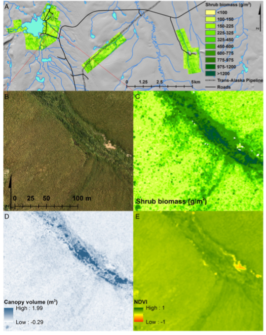
Figure 1. A: Overview of shrub biomass maps for the three LiDAR collection footprints (note biomass color scale is nonlinear). B-E: Enlarged view of a representative area showing B) RGB orthoimage for reference, C) Final shrub biomass map (color scale as in A), D) LiDAR-derived canopy volume at native resolution of 0.15m, and E) NDVI at native resolution of 0.043 m (Figure from Greaves et al., 2016).
Citation
Greaves, H.E., L. Vierling, J. Eitel, N. Boelman, T. Magney, C. Prager, and K. Griffin. 2018. High-Resolution Shrub Biomass and Uncertainty Maps, Toolik Lake Area, Alaska, 2013. ORNL DAAC, Oak Ridge, Tennessee, USA. https://doi.org/10.3334/ORNLDAAC/1573
Table of Contents
- Dataset Overview
- Data Characteristics
- Application and Derivation
- Quality Assessment
- Data Acquisition, Materials, and Methods
- Data Access
- References
Dataset Overview
This dataset contains estimates for aboveground shrub biomass and uncertainty at high spatial resolution (0.80-m) across three research areas near Toolik Lake, Alaska. The estimates for August of 2013 were generated and mapped using Random Forest modeling with input variables of optimized LiDAR-derived canopy volume and height, mean NDVI from 4-band RGB color and near-IR orthophotographs, and harvested biomass data. Uncertainty in the final shrub biomass maps was quantified by producing separate maps showing the coefficient of variation (CV) of the Random Forest map estimates. Shrub biomass was harvested at Toolik Lake in 2014 and used to optimize inputs and validate the final model and these biomass data are also provided.
Airborne LiDAR data and 4-band RGB color and near-IR digital imagery were collected August 1, 2013, over three separate research areas including a ~6-km2 area partially surrounding Toolik Lake, a ~3-km2 area surrounding upper Imnavait Creek, and a ~3-km2 area covering a section of the Trans Alaska Pipeline and surrounding terrain. The areas have different glacial histories but similar vegetation communities. Shrub biomass harvests were conducted in 2014 near the Toolik Lake Field Station at three 25-m radius areas. Harvest plot placement within these areas was chosen subjectively to capture a range of shrub species, biomass, density, and structure.
Related Publication:
Greaves, H.E., Vierling, L. A., Eitel, J.U.H, Boelman, N.T., Magney, T.S., Prager, C.M., & Griffin, K.L. (2016). High-resolution Mapping of Aboveground Shrub Biomass in Arctic Tundra Using Airborne Lidar and Imagery. Remote sensing of environment,(184), 361-373. http://dx.doi.org/10.1016/j.rse.2016.07.026
Related Datasets:
Greaves, H.E., J. Eitel, L. Vierling, N. Boelman, K. Griffin, T. Magney, and C. Prager. 2019. High-Resolution Vegetation Community Maps, Toolik Lake Area, Alaska, 2013-2015. ORNL DAAC, Oak Ridge, Tennessee, USA. https://doi.org/10.3334/ORNLDAAC/1690
Greaves, H.E., and E.A. Fortin. 2019. Ground-Based Vegetation Community Photos, Toolik Lake Area, Alaska, 2014-2015. ORNL DAAC, Oak Ridge, Tennessee, USA. https://doi.org/10.3334/ORNLDAAC/1718
Acknowledgements:
This work was supported by NASA Terrestrial Ecology grant NNX12AK83G, NASA Earth Science Fellowship NNX15AP04H awarded to HEG, and NASA Idaho Space Grant Fellowship NNX10AM75H awarded to TSM.
Data Characteristics
Spatial Coverage: The Toolik Lake area of the Alaskan North Slope
Spatial Resolution: 0.80-m
Temporal Coverage: 2013-08-01 to 2014-07-15
Temporal Resolution: One-time estimates
Study Areas (All latitude and longitude given in decimal degrees)
| Site | Westernmost Longitude | Easternmost Longitude | Northernmost Latitude | Southernmost Latitude |
|---|---|---|---|---|
| Toolik Lake area in Alaska | -149.6608333 | -149.2880556 | 68. 64388889 | 68. 61 |
Data file information
There are seven data files with this dataset: two files (one file of biomass data and one file with corresponding uncertainty data) in GeoTIFF (.tif) format for each of the three study areas, and one comma-separated (.csv) file with the biomass harvest data.
Table 1. Data file names and descriptions
| File name | Description |
|---|---|
| Toolik_Lake_Shrub_Biomass.csv | Dry shrub biomass including both stem and leaf material, provided in g/m2. |
| Toolik_Shrub_Biomass.tif | Mean shrub biomass estimates in g/m2 from all regression trees for each pixel for the research area partly surrounding Toolik Lake (an area of ~ 6 km2). |
| Toolik_Shrub_Biomass_uncertainty.tif | Shrub biomass estimate uncertainty for the the research area partly surrounding Toolik Lake (an area of ~ 6 km2). The map spatially illustrates the coefficient of variation of the shrub biomass estimates from all regression trees for each pixel, represented as a percentage of the estimated shrub biomass in each pixel. |
| Pipeline_Shrub_Biomass.tif | Mean shrub biomass estimates in g/m2 from all regression trees for each pixel for the research area covering a section of the Trans Alaska Pipeline (an area of ~ 3 km2). |
| Pipeline_Shrub_Biomass_uncertainty.tif | Shrub biomass estimate uncertainty for the research area covering a section of the Trans Alaska Pipeline (an area of ~ 3 km2). The map spatially illustrates the coefficient of variation of the shrub biomass estimates from all regression trees for each pixel, represented as a percentage of the estimated shrub biomass in each pixel. |
| Imnavait_Shrub_Biomass.tif | Mean shrub biomass estimates in g/m2 from all regression trees for each pixel for the research area surrounding upper Imnavait Creek (an area of ~ 3 km2 and ~10 km east of Toolik Lake). |
| Imnavait_Shrub_Biomass_uncertainty.tif | Shrub biomass estimate uncertainty for the Imnavait Creek research area (an area of ~ 3 km2 and ~10 km east of Toolik Lake). The map spatially illustrates the coefficient of variation of the shrub biomass estimates from all regression trees for each pixel, represented as a percentage of the estimated shrub biomass in each pixel. |
Table 2. Variables in the data file Toolik_Lake_Shrub_Biomass.csv
| Column | Units/format | Description |
|---|---|---|
| shrub_dry_mass | g/m2 | Shrub dry mass including both stem and leaf material in g/m2 |
| easting | Biomass harvest plot- Easting in NAD83 UTM 6N | |
| northing | Biomass harvest plot- Northing in NAD83 UTM 6N | |
| latitude | decimal degrees | Biomass harvest plot- center latitude |
| longitude | decimal degrees | Biomass harvest plot- center longitude |
| date | YYYY-MM-DD | Harvest collection date |
Table 3. Properties of the shrub biomass estimate GeoTIFF files
| File name | Units | Valid range | Mean value | Standard deviation | No-data value |
|---|---|---|---|---|---|
| Toolik_Shrub_Biomass.tif | g/m2 | 0-1559 | 247.1 | 230.5 | 2000 |
| Toolik_Shrub_Biomass_uncertainty.tif | % | 1-541 | 78 | 46.6 | 2000 |
| Pipeline_Shrub_Biomass.tif | g/m2 | 0-1552 | 259.2 | 189.1 | 2000 |
| Pipeline_Shrub_Biomass_uncertainty.tif | % | 16-487 | 75.1 | 38.9 | 2000 |
| Imnavait_Shrub_Biomass.tif | g/m2 | 0-1558 | 232.8 | 149.4 | 2000 |
| Imnavait_Shrub_Biomass_uncertainty.tif | % | 3-554 | 76.4 | 45.1 | 2000 |
Application and Derivation
This study presents a robust approach for using airborne LiDAR data and high-resolution airborne imagery to accurately map low-stature shrub biomass in Arctic tundra. The high-resolution shrub biomass maps produced in this study are a valuable baseline reference that will be useful to researchers seeking to understand tundra vegetation dynamics, or to improve estimates of carbon flux, nutrient cycling, and wildlife habitat in the rapidly changing tundra biome (Greaves et al., 2016).
Quality Assessment
The accuracy and validity of the maps were assessed by performing leave-one-out cross-validation for the main predictor and testing the resulting prediction relationship against a withheld dataset, and by providing out-of-bag error estimates and uncertainty maps for the final model.
The harvest plots did not include samples of the largest common shrub species (Salix alaxensis), which may limit the ability of the model to predict very high shrub biomass, or, by design, samples of shrubs less than 5 cm height. However, the shrub biomass maps capture a wider gradient of shrub cover and structure relative to previous work in this ecosystem (Greaves et al., 2016).
Data Acquisition, Materials, and Methods
Study area
There were three research areas in this study: one ~6 km2 area partly surrounding Toolik Lake (hereafter referred to as ‘Toolik’) that wraps around Toolik Lake from the northeast to southwest, one ~3 km2 area situated along the Trans-Alaska Pipeline where it crosses the high moraine ridge ~3 km east of Toolik Lake (‘Pipeline Ridge’), and one ~3 km2 area that covers much of the research area along Imnavait Creek, approximately 10 km east of Toolik Lake (‘Imnavait’). The areas have different glacial histories but similar vegetation communities.
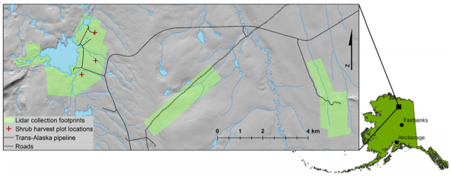
Figure 2. Location of study area in northern Alaska. Detail view shows three LiDAR collection footprints in pale green(from left to right: Toolik, PipelineRidge, Imnavait). Red crosses indicate locations of shrub harvest areas within the Toolik LiDAR footprint (Greaves et al., 2016).
Aboveground shrub biomass harvests
Shrub biomass harvests were conducted in 2014 at locations near the Toolik Lake Field Station (Figure 2). Three 25 m radius areas were selected, and 20 samples were collected from plots within each area. Harvest plot placement was chosen subjectively to capture a range of shrub species, biomass, density, and structure. Harvest plot center coordinates were measured with a TopCon GR-3 survey grade GPS system running in real time kinematic (RTK) mode (nominal accuracy 4 cm). A 0.64 m2 ring was placed at each harvest plot and all woody stems within greater than 5 cm height were identified. These woody stems were clipped to the moss layer and oven-dried at 50 °C until their mass measurements stabilized (generally >48 h), then weighed to the nearest tenth of a gram to determine total dry shrub biomass per plot. Dry shrub biomass included both stem and leaf material. All shrub species were pooled for analysis, but visual assessment suggested that species contributing the majority of biomass included Salix pulchra Cham., S. richardsonii Hook., S. glauca L., Betula nana L., and Vaccinium uliginosum L.
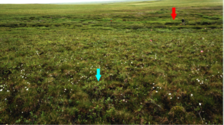
Figure 3. Example of complex tundra microtopography and absence of ‘bare earth’ showing low-stature shrubs (~ 0.25 m; example indicated with blue arrow) growing among cottongrass tussocks and moss in the foreground, and hummocks with larger shrubs (~ 0.80–1 m); example is indicated with red arrow in the middle distance. Photo was taken near the detail image shown in Fig.1, B–E. A reflective target at the upper center (tripod with red circle, ~ 2-m tall) and a person near the red arrow provide scale (Greaves et al., 2016).
Airborne LiDAR and imagery collection
Airborne LiDAR data (approximate point density of 30 points/m2) and digital imagery were collected August 1st, 2013, in three separate footprints. See Vierling et al. (2013a) for access to LiDAR data in *.las format. For this study, all laser returns were included in analyses (i.e. data were not filtered based on return numbers, return intensities, or scan angles).
Simultaneous 4-band digital imagery (RGB and near infrared, hereafter ‘RGB-NIR’) was collected with a Leica RCD30 60MP camera mounted to the aircraft, and was processed and orthorectified to create orthoimagery mosaics with a pixel resolution of 4.25-cm. A GPS spot-check of 40 stationary objects distributed across the Toolik data collection footprint suggested that the imagery was accurately orthorectified to within 10 cm. See Vierling et al. (2013b) for access to the orthophotographs.
Lidar canopy volume processing
A rasterized canopy volume map was created using an optimization algorithm based on previous work with terrestrial LiDAR (Greaves et al., 2015). To produce canopy volume, the algorithm iteratively alters search parameters that are used to classify and rasterize laser returns. The lowest and highest LiDAR laser returns were interpolated and rasterized. Canopy volume rasters were subsequently aggregated to 0.80-m resolution to match the area of the shrub harvest plots. The strength of the relationship between optimized canopy volume and harvested shrub biomass was characterized using the coefficient of determination (R2) and root mean squared error (RMSE). To evaluate the predictive strength of this simple model, the model was applied to predict biomass for a stratified-random sample of harvested shrubs that had been withheld from the optimization algorithm (i.e. a test dataset, n = 20). The optimized set of classification parameters was applied to all LiDAR returns to create wall-to-wall canopy volume rasters for the three LiDAR footprints. These canopy volumes are unlikely to be accurate in absolute terms because of the difficulty in identifying bare earth and canopy surfaces in shrubby areas.
Additional LiDAR canopy metrics
The optimized ground points were used to pseudo-normalize vegetation return heights in LAStools (the term ‘pseudo-normalize’ is used to acknowledge the shortcomings of using the optimized surfaces for this purpose). These height-normalized point clouds were further processed in LAStools to create layers representing maximum estimated canopy height, vegetation density, and standard deviation of maximum heights. These layers were produced at 0.80 m resolution using a 0.05 m vegetation height threshold, to match the area and harvest protocol of our shrub harvest plots (Greaves et al., 2016).
Spectral metrics
Maximum and mean values for NDVI were calculated from the aerial RGB-NIR images at 0.80 m resolution, and averaged over 2.4 m to incorporate information from surrounding vegetation.
Random Forest regression
The biomass maps in this dataset were generated from a Random Forest model built using both spectral data and lidar-derived canopy data. Because the stochastic nature of Random Forest can give different results with each execution of the algorithm, the model selection tool was run 1,000 times for each model (the canopy and spectral model), and only included predictors in the final Random Forest models if they were chosen in a majority of the variable selection runs. The important predictors selected included optimized canopy volume, maximum canopy height, standard deviation of maximum canopy height, and mean NDVI.
Biomass mapping
Biomass predictor rasters were processed using the R package ‘raster’, and biomass was mapped at 0.80 m across the LiDAR footprints using the AsciiGridPredict tool in the R package ‘yaImpute’ (Crookston and Finley, 2007). In the final shrub biomass maps, the shrub biomass estimate for a given pixel is the mean of all estimates produced by all regression trees for that pixel. Because the focus of map production was to identify shrub biomass (even very low-stature shrub biomass) in uneven terrain, filtering was not performed to identify ‘unnatural’ ground slopes or to mask non-vegetation objects other than roads and large gravel pads; consequently, the maps contain spurious values for objects on the landscape such as boardwalks and research equipment (e.g. greenhouses and eddy covariance towers). However, these objects are generally recognizable to the human eye based on their linearity or improbable height or position and can be manually masked in areas of interest if necessary.
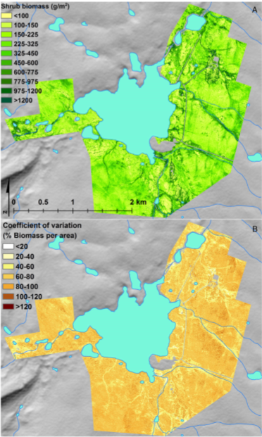
Figure 4. Shrub biomass estimates (A) and coefficient of variation of shrub biomass estimates (B) for the Toolik collection footprint (Greaves et al., 2016).
Uncertainty
Uncertainty was quantified in the final shrub biomass map by producing a separate map showing the coefficient of variation (CV) of the Random Forest map estimates. The individual pixel estimates from all trees were retained and the standard deviation of each pixel estimate was calculated across all trees. Normalizing this per-pixel standard deviation by the per-pixel mean gives the per pixel coefficient of variation. The resulting CV map spatially illustrates the variation of the model estimates, represented as a percentage of the estimated shrub biomass in each pixel.
Data Access
These data are available through the Oak Ridge National Laboratory (ORNL) Distributed Active Archive Center (DAAC).
High-Resolution Shrub Biomass and Uncertainty Maps, Toolik Lake Area, Alaska, 2013
Contact for Data Center Access Information:
- E-mail: uso@daac.ornl.gov
- Telephone: +1 (865) 241-3952
References
Crookston, N.L. and A.O. Finley. 2007. yalmpute: an R package for K-NN imputation. J. Stat. Softw. 23 (10), 1-16.
Greaves, H.E., Vierling, L. A., Eitel, J.U.H, Boelman, N.T., Magney, T.S., Prager, C.M., & Griffin, K.L. (2016). High-resolution Mapping of Aboveground Shrub Biomass in Arctic Tundra Using Airborne Lidar and Imagery. Remote sensing of environment,(184), 361-373. http://dx.doi.org/10.1016/j.rse.2016.07.026
Greaves, H.E., Vierling, L. A., Eitel, J.U.H, Boelman, N.T., Magney, T.S., Prager, C.M., & Griffin, K.L. (2015). Estimating Aboveground Biomass and Leaf Area of Low-Stature Arctic Shrubs with Terrestrial LiDAR. Remote sensing of environment, (164), 26-35. https://doi.org/10.1016/j.rse.2015.02.023
Vierling, L.A., Eitel, J.U.H., Boelman, N.T., Griffin, K.L., Greaves, H., Magney, T.S., Prager, C., Ajayi, M., and Gibson, R. 2013a. Bare earth LiDAR dataset for Toolik Field Station, AK, and nearby field sites along Dalton Highway. https://doi.org/10.7923/G4057CV5
Vierling, L.A., Eitel, J.U.H., Boelman, N.T., Griffin, K.L., Greaves, H., Magney, T.S., Prager, C., Ajayi, M., and Gibson, R. 2013b. Four-band, 5 cm Resolution Orthophotographs of Toolik Field Station, AK, and Nearby Field Sites Along Dalton Highway. http://dx.doi.org/10.7923/G4VD6WCW