Documentation Revision Date: 2026-02-05
Dataset Version: 1
Summary
This dataset includes 11 files: six landcover maps as Cloud-optimized GeoTIFFs (COGs), field data in a shapefile and a comma separated values (CSV) file, two text files with recommended color schemes for displaying the COGs, and an associated report in PDF format.
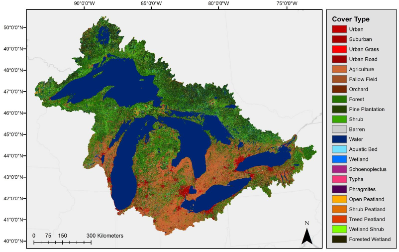
Figure 1. Landcover and wetland type map of the Great Lakes Basin.
Citation
Bourgeau-Chavez, L.L., M.J. Battaglia, M.E. Miller, J.A. Graham, A.F. Poley, and D.J.L. Vander Bilt. 2026. Baseline Wetland Type and Land Cover Map of the Great Lakes Basin, 2010. ORNL DAAC, Oak Ridge, Tennessee, USA. https://doi.org/10.3334/ORNLDAAC/2440
Table of Contents
- Dataset Overview
- Data Characteristics
- Application and Derivation
- Quality Assessment
- Data Acquisition, Materials, and Methods
- Data Access
- References
Dataset Overview
This dataset holds maps of land cover and wetland ecotype for the Great Lakes Basin (GLB) circa 2010. The data were derived from multi-season L-band SAR, Landsat 5 optical imagery, and thousands of field training data samples. The dataset includes detailed landcover maps of shorelines of each of five Great Lakes along with a land cover map of the entire GLB. This is the first binational map of the GLB that specifically depicts native wetland ecotypes and monocultures of invasive wetland plants (Phragmites australis and Typha spp.). The goal of the effort was to improve understanding of nutrient flow and transport of water across the landscape to the coasts and the processes at the land-water interface in wetland ecosystems that lead to the success of invasive species. An associated report is included in PDF format.
Project: Vegetation Collection
The ORNL DAAC compiles, archives, and distributes data on vegetation from local to global scales. Specific topic areas include: belowground vegetation characteristics and roots, vegetation biomass, fire and other disturbance, vegetation dynamics, land cover and land use change, vegetation characteristics, and NPP (Net Primary Production) data.
Related Dataset:
Bourgeau-Chavez, L.L., S. Endres, M. Battaglia, and E. Banda. 2017. NACP Peatland Land Cover Map of Upper Peninsula, Michigan, 2007-2011. ORNL DAAC, Oak Ridge, Tennessee, USA. https://doi.org/10.3334/ORNLDAAC/1513
Acknowledgements:
The research was supported by NASA's Interdisciplinary Research in Earth Science (IDS) program (grants 80NSSC17K0262, NNX11AC72G).
Data Characteristics
Spatial Coverage: Great Lakes Basin, Canada and United States
Spatial Resolution: 12.5 m
Temporal Coverage: 2007-04-01 to 2011-04-15: map products circa 2010
Temporal Resolution: One time estimate
Site Boundaries: Latitude and longitude are given in decimal degrees.
| Site | Westernmost Longitude | Easternmost Longitude | Northernmost Latitude | Southernmost Latitude |
|---|---|---|---|---|
| Great Lakes Basin, Canada and United States |
-97.2812 | -71.5680 | 52.5535 | 38.7120 |
Data File Information
This dataset holds 10 files: six landcover maps as cloud optimized GeoTIFFs (Table 1), field data in a shapefile and a CSV file, two text files with recommended color schemes for displaying the GeoTIFFs, and an associated report in PDF format.
GeoTIFF characteristics:
- Coordinate system: UTM zones 16N and 17N (EPSG: 32616, 32617), WGS 84 datum, units = meters.
- Spatial resolution: 12.5 m
- Data type: Byte
- Pixel values: landcover classes and wetland types (Table 2)
Table 1. GeoTIFF files and relevant metadata.
| File name | Spatial extent | UTM zone | Nodata value |
|---|---|---|---|
| GLB_landcover_complete_v4.tif | The entire Great Lakes Basin (Figure 1) | 17 | 127 |
| GLB_landcover_lake_erie.tif, GLB_landcover_lake_huron.tif, GLB_landcover_lake_michigan.tif, GLB_landcover_lake_ontario.tif, GLB_landcover_lake_superior.tif |
Shorelines along each respective Great Lake | 16 | 255 |
Two files holding the recommended color table for effective display of the GeoTIFFs in GIS software. Use GLB_landcover_Colormap.clr for ArcGIS and GLB_landcover_Colormap.qmd for QGIS.
GLB_landcover_field_points.zip is a compressed archive holding a shapefile with field data and sampling locations. The same information is available in the CSV file, GLB_landcover_field_data.csv. (See attributes in Table 3).
In the CSV, missing data are indicated by "NA" for text fields and "-9999" for numeric fields.
In the CSV, four sampling locations lack longitude-latitude coordinates; those points are not included in the shapefile.
GLB_landcover_WriteUp.pdf is a report detailing the methods and accuracy assessment.
Table 2. Pixel values with descriptions in GeoTIFFs.
| Value | Description |
|---|---|
| 1 | Urban |
| 2 | Suburban |
| 3 | Urban Grass |
| 4 | Urban Road |
| 5 | Agriculture |
| 6 | Fallow Field |
| 7 | Orchard |
| 8 | Forest |
| 9 | Pine Plantation |
| 10 | Shrub |
| 11 | Barren Light |
| 12 | Barren Dark |
| 13 | Water |
| 14 | Aquatic Bed |
| 15 | Wetland |
| 16 | Schoenoplectus |
| 17 | Typha |
| 18 | Phragmites |
| 20 | Open Peatland |
| 21 | Shrub Peatland |
| 22 | Treed Peatland |
| 23 | Shrub Wetland |
| 24 | Forested Wetland |
Table 3. Attribute fields in the GLB_landcover_field_points.zip (shapefile) and GLB_landcover_field_data.csv (CSV).
| Variable name | Units | Brief Description | |
|---|---|---|---|
| CSV | Shapefile | ||
| geodjango_group | geodjango_ | Project for which the data were collected if applicable (i.e. USGS, NASA IDS, EPA, USFWS) | |
| id | id | 1 | Unique ID for each entry |
| lowest_branch_height_m | low_branch | m | For treed plots, a measure of the height of the lowest living branch |
| direct_access | direct_acc | Whether plot was monitored directly within the wetland (t = true) or from remote location (false) | |
| complex_name | complex_nm | Wetland complex name given for field organization purposes | |
| waypoint_id | waypt_id | 1 | GPS waypoint ID |
| opportunistic | opportun | Whether plot selection was opportunistic (t = true, f = false) or planned. | |
| visit_date | visit_date | YYYY-MM-DD | Date of plot visit |
| water_level_value | water_lev | cm | Height of the water from bottom to surface at time of visit |
| waterlevel_time | water_time | hh:mm | Time of the water level measurement |
| site_access_notes | access_not | Plot access notes | |
| gps_time | gps_time | hh:mm:ss | Time of GPS coordinate acquisition |
| ecosystem_type_id | ecosys_id | 1 | Unique number given to each ecosystem type |
| ecosystem_type_comments | ecosys_com | Ecosystem type (emergent wetland, open water, floating aquatic, etc) | |
| stand_type_id | stand_type | 1 | ID given to plot type (1-3) |
| stand_type_name | stand_nam | Whether the plot sampled was pure monotypic, mixed with less than 6 vascular species, or missed with more than 6 vascular species | |
| dominant_species_id | dom_sp_id | 1 | Unique ID given to dominant vegetation species present |
| dominant_species_common_name | dom_sp_nam | Common name of the dominant vegetation species present | |
| species_distribution_id | sp_dist_id | 1 | Unique number given to species distribution (1,2, or 99) |
| species_distribution_name | sp_dist_nm | Species distribution (patchy, evenly mixed or other) | |
| phrag_present_flag | phrag_pres | Was invasive Phragmites australis present | |
| phrag_pcnt_cover | phrag_covr | 1 | Visual estimate of percent invasive Phragmites present |
| phrag_condition_id | phrag_cond | 1 | Unique number given to each Phragmites condition |
| phrag_condition_name | phrag_name | Condition of the Phragmites (untreated, burned, mowed, chemically treated, other) | |
| homogeneity_dense_veg_pcnt_cover | h_dens_cov | 1 | Visual estimate of percent cover of dense vegetation in the plot |
| homogeneity_sparse_veg_pcnt_cover | h_spar_cov | 1 | Visual estimate of percent cover of exposed mud in the plot |
| homogeneity_mud_flats_pcnt_cover | h_mudf_cov | 1 | Visual estimate of percent cover of sparse vegetation in the plot |
| homogeneity_open_water_pcnt_cover | h_watr_cov | 1 | Visual estimate of percent cover of open water in the plot |
| homogeneity_other_pcnt_cover | h_othr_cov | 1 | Visual estimate of percent cover of other condition in the plot |
| homogeneity_other_comments | h_othr_com | Description of the "other percent cover" in the plot | |
| latitude | latitude | degrees north | Latitude of point in decimal degrees |
| longitude | longitude | degrees east | Longitude of point in decimal degrees |
Application and Derivation
Previous research resulted in a circa 2010 bi-national map of coastal land cover and wetland types in the Great Lakes at moderate resolution (~20 m) within 10 km of the coastline which was produced for the Great Lakes Restoration Initiative. The coastal map and two other maps of interior Michigan were created for each 70 km x 70 km area of interest (defined by ALOS PALSAR FBD scenes) with field data collected within that perimeter (Bourgeau-Chavez et al., 2015; Bourgeau-Chavez et al., 2017).
This dataset provides a full basin map that was completed using transfer learning of training data with minimal new field data. It is a single map crossing the international border using the same input remote sensing datasets (three season PALSAR and Landsat-5). The sections of the map produced with field training data collected within each AOI have higher map accuracy than those areas with transfer learning,
Quality Assessment
Classification accuracy was assessed by comparing classified covers to ground-truth values via confusion matrix. The overall accuracy was 81%. See details in the GLB_landcover_WriteUp.pdf.
Data Acquisition, Materials, and Methods
The study area spans the entirety of the Laurentian Great Lakes Basin, which includes the entire state of Michigan, portions of Minnesota, Wisconsin, Illinois, Indiana, Ohio, Pennsylvania and New York, and parts of the Canadian province of Ontario. Areas mapped under previous projects, which include areas within 10 km from the of the Great Lakes’ shoreline and the state of Michigan, were used as sources of training data, while the targets of mapping for this study focused on the rest of the basin, which consists of all areas further than 10 km inland from the shoreline of the Lakes (Figure 1).
Image Data
Following Bourgeau-Chavez et al. (2015), each area of interest required LANDSAT 5 TM and ALOS PALSAR data representing spring, summer, and autumn time frames. April and May images were categorized as spring, June, July, and August images were considered summer, and September and October images were used to represent autumn. Slight adjustments were made for areas of interest (AOI) further north, where a colder climate causes spring to arrive later. Images collected during the 2010 calendar year were prioritized, and images from 2007-2011 were used when 2010 images were not available.
LANDSAT 5 TM images were selected based on lack of clouds and haze. Optical bands were processed to top-of-atmosphere reflectance and thermal bands were converted to top-of-atmosphere brightness temperature in degrees Celsius. Normalized Difference Vegetation Index (NDVI) was also calculated for each image using the red (band 3) and near-infrared (band 4) bands. Images were resampled to 12.5-meter spatial resolution using a nearest neighbor resampling approach in order to match the resolution of the PALSAR data. In some cases, a cloud-free image was unavailable and two images were combined to create one cloud-free composite image. When this occurred, the QA band was used to detect pixels that had cloud contamination in the primary image (typically the image with less overall cloud cover), and those pixels were replaced with cloud free pixels from the secondary image.
Radiometrically terrain corrected (RTC) ALOS PALSAR data were acquired from NASA’s Alaska Satellite Facility (ASF). Fine Beam Dual (FBD) mode data, which contains both co-polarized and cross-polarized backscatter, were used whenever available. When FBD was not available, Fine Beam Single (FBS, HH only) mode was used. The FBD and FBS RTC images are provided in gamma-nought backscatter and are terrain corrected to eliminate geometric distortions caused by varying topography (Small, 2011). To make these images consistent with the PALSAR imagery used for the coastal and Michigan maps, the images were converted to sigma-nought backscatter using the following equation: σ0 = γ0 x cos θ
After images were converted to sigma-nought, they were filtered to remove speckle noise using a 3x3 median filter. Although the radiometric terrain correction products exhibited relatively few geolocation issues, images were checked for co-registration errors. Images with more than 1 pixel off-set were georeferenced manually using overlapping LANDSAT 5 TM imagery as the reference dataset.
In addition to the seasonal LANDSAT 5 TM and PALSAR images, topographic position indices (TPI) were derived using digital elevation models and included in data stacks for classification. TPI has been shown to be a valuable variable for wetland classification in a variety of studies. For the United States portion of the GLB, 1/3 arc second DEMs from the USGS 3DEP program were used. For Canada, SRTM data was used. Topographic position index provides a simple index to indicate relative position of an individual pixel in relation to a user defined neighborhood (Weiss, 2001); circular neighborhoods with 75 pixel and 200 pixel radii were used.
Data stacks containing the triplicates of LANDSAT 5 TM and PALSAR and the two TPI layers were generated for all unmapped areas in the GLB using 70 km x 70 km PALSAR scene extents to define AOIs. When the PALSAR extents were not completely within a LANDSAT path/row, it was split into two separate AOIs according to the overlapping LANDSAT scenes. In total, data stacks for 266 AOIs were generated.
To account for regional variability in vegetation types, AOIs were partitioned as follows: AOIs were first subdivided into groups to represent ecoregions with similar vegetation composition, geology, and soil types. These groups were then further subdivided into smaller contiguous regions based on longitudinal or latitudinal gradients so that each grouping contained adequate source training data, which was set to be at least 10 AOIs. Each AOI was finally categorized as a source, meaning it had been previously mapped and had training polygons available, or a target, meaning it was unmapped and had no training polygons available within its boundaries (Table 4, Figure 2).
Table 4. Number of areas of interest (AOI) in each region.
| Region | Source AOI | Target AOI |
|---|---|---|
| Eastern_Temp_Forest_Central_N | 43 | 9 |
| Eastern_Temp_Forest_Central_S | 10 | 20 |
| Eastern_Temp_Forest_West_N | 24 | 23 |
| Eastern_Temp_Forest_West_S | 29 | 16 |
| Mixed_Wood_Plains_East | 40 | 52 |
| Mixed_Wood_Shield_Central | 44 | 14 |
| Mixed_Wood_Shield_East | 11 | 46 |
| Mixed_Wood_Shield_West | 42 | 40 |
| Softwood_Shield_North | 13 | 46 |
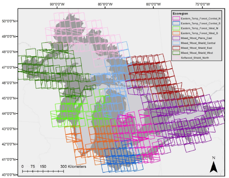
Figure 2. PALSAR and LANDSAT defined areas of interest (AOI) grouped according to ecoregions.
Temporal variability of image data required further selection criteria of input imagery to derive training data for target AOIs. Plants in early spring imagery were likely to be at a different phenological state than plants within the same map category imaged later in spring (Figure 3). To account for the impact of phenology, training data from available source AOIs for each target AOI were selected by matching NDVI values of deciduous forest. Deciduous forests are distributed across the GLB and were assumed to be good indicators of scene-wide vegetation condition and appropriate for comparison between AOIs (Figure 4).
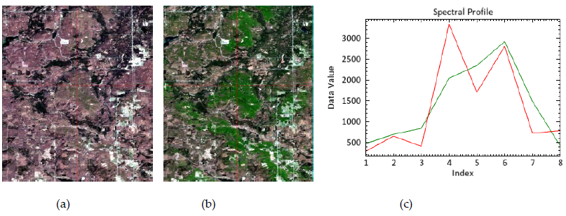
Figure 3. Phenological change due to leaf out in Spring for two Landsat-5 TM images near Lewiston, Michigan: (a) 2010-04-23, (b) 2010-05-09. The spectral profile (c) illustrates differences in same pixel between two images. Green line represents (a) and the red line represents (b). TOA reflectance values on the y-axis are scaled by 10,000.
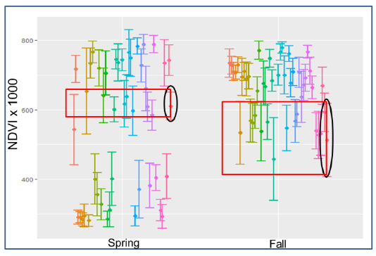
Figure 4. Mean NDVI values in deciduous forest samples the Mixed Wood Shield ecoregion for example target AOI (circled in black) and source AOIs (multicolored dots) for spring and fall Landsat imagery.
Mapping Technique
Only source AOIs with both matching spring and autumn NDVI values were used to train the models for classifying target AOIs. Once the source AOIs were identified, each pixel within their respective training polygons were gathered as training samples. Values for each pixel for each of the 38 input data bands were aggregated into a large training dataset used as input into the classifier. The classification procedure was implemented in R software using the randomForest package. The classifier was parameterized to use 500 unique trees for each model which were then used to predict the unique class for each pixel within the target AOI data stack. The classified maps for each target AOI were mosaicked together. In overlapping areas, visual inspection was used to determine which output would be placed on top.
Validation and accuracy assessment
The classified map was compared to field data and aerial photographs. Field data from as close to 2010 as possible were used to ensure it was representative of conditions in 2010. Field visits were conducted during 2018 and included 196 wetland sites, mostly located in Wisconsin, New York, and Ontario. An additional 71 field verified locations were acquired from collaborators at Environment and Climate Change Canada, representing wetlands within the Lake Huron, Lake Erie, and Lake Ontario watersheds (Figure 5).
Additional validation data were also generated using air photo interpretation methods with historical imagery from USDA NAIP imagery collections, where available, in order to attain adequate spatial distribution across the basin. Validation polygons digitized using image interpretation represented all land cover types, including wetlands, uplands, and developed classes. In total, 958 polygons derived from image interpretation were used in addition to the 267 field verified wetland polygons. Each polygon represented a homogenous area on the ground of at least .2 hectares, which was determined to be the minimum mapping unit (Bourgeau-Chavez et al, 2015). The validation polygons were used to generate error matrices, which quantified the number of correctly and incorrectly classified pixels within each polygon on a class-by-class basis.
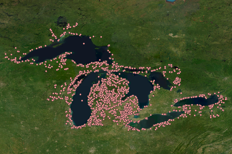
Figure 5. Locations of field sites represented in GLB_landcover_field_points.zip (shapefile) and GLB_landcover_field_data.csv.
See Battaglia et al.(2025, file GLB_landcover_WriteUp.pdf) for additional details.
Data Access
These data are available through the Oak Ridge National Laboratory (ORNL) Distributed Active Archive Center (DAAC).
Baseline Wetland Type and Land Cover Map of the Great Lakes Basin, 2010
Contact for Data Center Access Information:
- E-mail: uso@daac.ornl.gov
- Telephone: +1 (865) 241-3952
References
Battaglia, M.J., M.E. Miller, J. Graham, A. Poley, D.J.L. Vander Bilt, and L. Bourgeau-Chavez. 2025. Expansion of a baseline wetland type and land cover map for the GLB using training-data transfer methods. (an unpublished report included with this dataset; file GLB_landcover_WriteUp.pdf)
Bourgeau-Chavez, L., S. Endres, M. Battaglia, M. Miller, E. Banda, Z. Laubach, P. Higman, P. Chow-Fraser, and J. Marcaccio. 2015. Development of a Bi-National Great Lakes Coastal Wetland and Land Use Map Using Three-Season PALSAR and Landsat Imagery. Remote Sensing 7:8655-8682. https://doi.org/10.3390/rs70708655
Small, D. 2011. Flattening Gamma: Radiometric Terrain Correction for SAR Imagery. IEEE Transactions on Geoscience and Remote Sensing 49:3081-3093. https://doi.org/10.1109/tgrs.2011.2120616
Weiss, A. 2001. Topographic position and landforms analysis. In Proceedings of the Poster presentation, ESRI user conference, San Diego, CA, 9-13 July 2001.