Documentation Revision Date: 2018-07-30
Data Set Version: 1
Summary
There are 60 data files in GeoTIFF (.tif) format and one data file in comma-separated (.csv) format with this dataset. The GeoTIFF files provide carbon consumption and consumption uncertainties separately for each of the 29 ABoVE reference grid tiles for the NWT domain. There is also a consumption data file and an uncertainty data file covering the entire domain. The .csv file provides plot characteristics, soil carbon, and estimated carbon combustion data.
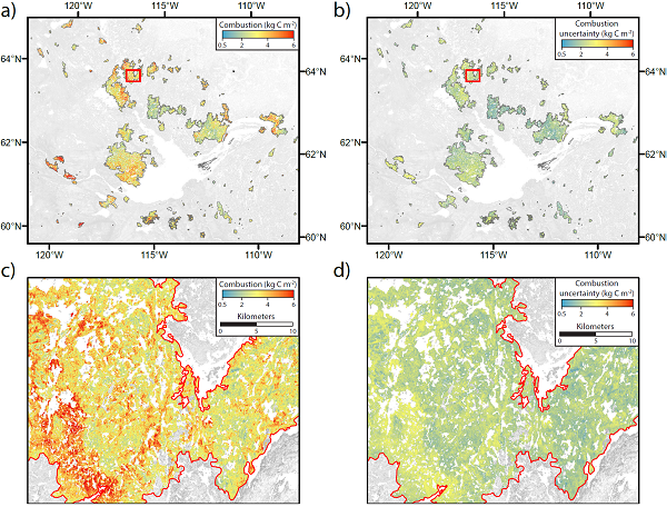
Figure 1. Maps of the 2014 NWT fire complex showing a) estimated total combustion, b) uncertainty in total combustion, and details of landscape heterogeneity in c) combustion and d) uncertainty within one of the major fire scars. From Walker et al., 2018.
Citation
Walker, X.J., B.M. Rogers, J.L. Baltzer, S.R. Cummings, N.J. Day, S.J. Goetz, J.F. Johnstone, M.R. Turetsky, and M.C. Mack. 2018. ABoVE: Wildfire Carbon Emissions and Burned Plot Characteristics, NWT, CA, 2014-2016. ORNL DAAC, Oak Ridge, Tennessee, USA. https://doi.org/10.3334/ORNLDAAC/1561
Table of Contents
- Data Set Overview
- Data Characteristics
- Application and Derivation
- Quality Assessment
- Data Acquisition, Materials, and Methods
- Data Access
- References
Data Set Overview
The focus of this study was to develop a high spatial resolution model to scale emissions from fires that occurred near Yellowknife, Northwest Territories, Canada, during 2014. A model was derived using only covariates obtainable from geospatial layers that covered the entire spatial domain of interest. The final model was used to estimate total C emissions at 30-m resolution across all fires in the 2014 NWT fire complex.
To apply the model across all fire perimeters, final model covariates were re-gridded to a common 30-m grid and Canadian Albers Equal Area Conic projection defined by 29 tiles within the ABoVE 30-m reference grid (Loboda et al., 2017). The regression model was then applied to burned pixels defined by a threshold of Landsat-derived differenced Normalized Burn Ratio (dNBR) within fire perimeters.
A Monte Carlo framework was adopted to quantify predictive uncertainty assumed to arise from measurement error in aboveground and belowground combustion, and landscape scaling.
Plot data collected at the wildfire burned sites and from unburned sites with similar characteristics are also included with this dataset. The plot data include site characteristics, tree cover and species, basal area, dNBR, plot characteristics, soil carbon, and carbon combusted. Combustion related data were not collected at unburned plots.
Project: Arctic-Boreal Vulnerability Experiment
The Arctic-Boreal Vulnerability Experiment (ABoVE) is a NASA Terrestrial Ecology Program field campaign based in Alaska and western Canada between 2016 and 2021. Research for ABoVE links field-based, process-level studies with geospatial data products derived from airborne and satellite sensors, providing a foundation for improving the analysis and modeling capabilities needed to understand and predict ecosystem responses and societal implications.
Related Datasets:
Bourgeau-Chavez, L.L., S. Endres, L. Jenkins, M. Battaglia, E. Serocki, and M. Billmire. 2017. ABoVE: Burn Severity, Fire Progression, and Field Data, NWT, Canada, 2015-2016. ORNL DAAC, Oak Ridge, Tennessee, USA. https://doi.org/10.3334/ORNLDAAC/1548
Bourgeau-Chavez, L.L., N.H.F. French, S. Endres, L. Jenkins, M. Battaglia, E. Serocki, and M. Billmire. 2016. ABoVE: Burn Severity, Fire Progression, Landcover and Field Data, NWT, Canada, 2014. ORNL DAAC, Oak Ridge, Tennessee, USA. http://dx.doi.org/10.3334/ORNLDAAC/1307
Loboda, T.V., E.E. Hoy, and M.L. Carroll. 2017. ABoVE: Study Domain and Standard Reference Grids. ORNL DAAC, Oak Ridge, Tennessee, USA. http://dx.doi.org/10.3334/ORNLDAAC/1367
Veraverbeke, S., Rogers, B. M., Goulden, M. L., Jandt, R., Miller, C. E., Wiggins, E. B., & Randerson, J. T. (2017). ABoVE: Ignitions, burned area and emissions of fires in AK, YT, and NWT, 2001-2015. ORNL DAAC. https://doi.org/10.3334/ORNLDAAC/1341
Acknowledgements: This research was performed with support from NASA ABoVE, Grant NNX15AT71A.
Data Characteristics
Spatial Coverage: Northwest Territories, Canada
ABoVE Reference Locations:
Domain: Core ABoVE
State/territory: Northwest Territories (NWT), Canada
Grid cells: Ah1v1Bh4v0, Ah1v1Bh4v1, Ah1v1Bh4v4, Ah1v1Bh5v0, Ah1v1Bh5v1, Ah1v1Bh5v2, Ah1v1Bh5v3, Ah1v1Bh5v4, Ah1v1Bh5v5, Ah1v2Bh5v0, Ah2v1Bh0v3, Ah2v1Bh0v4, Ah2v1Bh0v5, Ah2v1Bh1v2, Ah2v1Bh1v3, Ah2v1Bh1v4, Ah2v1Bh1v5, Ah2v1Bh2v3, Ah2v1Bh2v4, Ah2v1Bh2v5, Ah2v1Bh3v5, Ah2v1Bh4v5, Ah2v2Bh0v0, Ah2v2Bh1v0, Ah2v2Bh2v0, Ah2v2Bh2v1, Ah2v2Bh3v0, Ah2v2Bh4v0, Ah2v2Bh4v1
Spatial Resolution: 30 meters and multiple points (field data)
Temporal Coverage: 2014-07-02 to 2016-08-01
Temporal Resolution: One time
Study Areas (All latitude and longitude given in decimal degrees)
| Site | Westernmost Longitude | Easternmost Longitude | Northernmost Latitude | Southernmost Latitude |
|---|---|---|---|---|
| Northwest Territories, CA | -136.119 | -102 | 71.69472 | 56.25417 |
Data file information
There are 60 data files in GeoTIFF (.tif) format with this dataset. This includes one aggregated file for carbon emissions and one aggregated file for uncertainty across the entire study domain, plus files for estimated carbon emissions and uncertainties for each of the 29 grid cells. The grid locations are included in the file names. Emissions data are provided in units of g C/m2.
There is also one file in comma-separated format which provides the field data collected at burned and unburned sites.
The 30-m (B-grid) tiles in the ABoVE grid are the small tiles nested inside the larger (A-grid) 240-m tiles in Figure 2. The first part of the grid cell name refers to the large A-grid, the second part refers to the B-grid. The correct tile is located by first locating the larger grid named AhAv, and then locating the smaller tile named BhBv within the larger tile. Examples are provided below in the last two file descriptions.
Table 1. File names and descriptions.
| File name | Description |
|---|---|
| Carbon_consumption_domain.tif | One aggregated data file for carbon consumption (g C/m2) over entire wildfire area. |
| Carbon_uncertainty_domain.tif | One aggregated data file for predicted carbon consumption uncertainty (g C/m2) over entire wildfire area. |
| Carbon_consumption_AhXvX_BhYvY.tif |
Carbon consumption (g C/m2) in the ABoVE tile number AhXvX_BhYvY |
| Carbon_uncertainty_AhXvX_BhYvY.tif |
Prediction uncertainty of carbon consumption (g C/m2) in the ABoVE tile number AhXvX_BhYvY Example file name: Carbon_uncertainty_Ah2v1_Bh0v5.tif. This is the lower tile marked with a yellow X in Figure 2 |
|
NWT_site_charac_combustion.csv
|
This file provides burned and unburned plot characteristics, tree basal area and species coverage, soil carbon, moisture, and estimated carbon combustion data. Refer to Table 2. for the variables and descriptions. The plot measurements were collected between June 2015 and June 2016 from burned and unburned sites. |
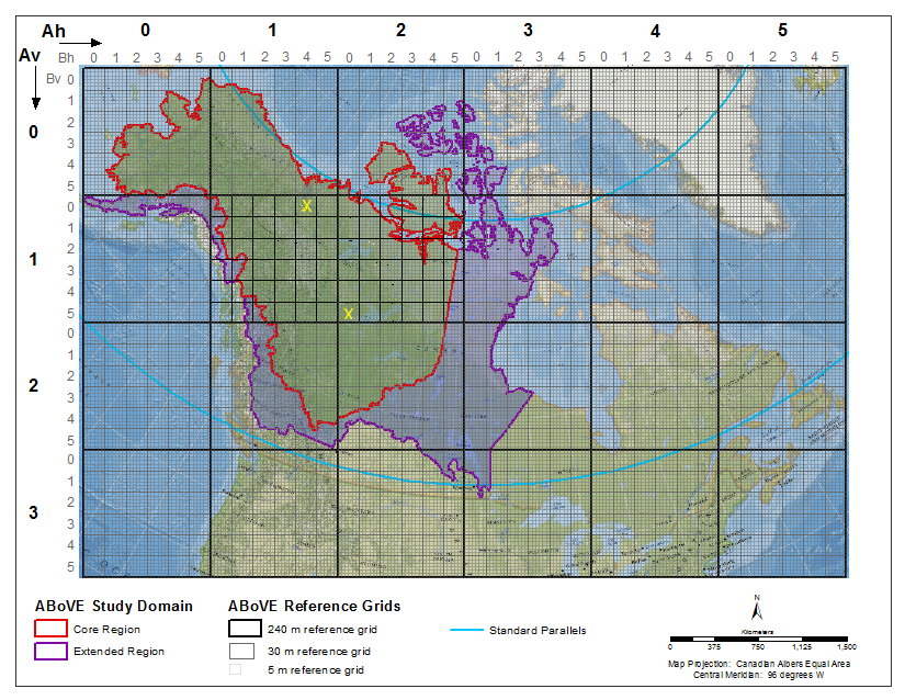
Figure 2. The ABoVE reference grid and study domain. The 240-m reference grid (4,500 X 4,500 grid cells per tile) with associated Ah and Av values, and the 30-m reference grid (6,000 X 6,000 grid cells per tile) superimposed on the 240-m grid with associated Bh and Bv values (Loboda et al., 2017). The yellow Xs indicate the tiles from the data files in the examples above.
Table 2. Variables in the file NWT_site_charac_combustion.csv
The data are from 211 burned and 36 unburned sites. All measurements were not made at the unburned sites as they did not apply (post fire measurements combustion data, etc). Missing data or data not applicable are recorded as -9999.
| Variable | Units/format | Description |
|---|---|---|
| site | Site name | |
| plot | Plot name | |
| burn | Name of the Burn Scar or Unburned area (SS33=Kakisa, ZF20=CentralHwy3, ZF46=NorthernHwy3, ZF35=Gameti West, ZF44=Gameti East, ZF26=Wekweeti, ZF104-Discovery Mine, CS= Control Shield, CG1 = Control Group 1, CG2 = Control Group 2) | |
| lat_start | decimal degrees | Latitude at start of west transect from GPS. Datum: WSG84 Position format: hddd.ddddd |
| long_start | decimal degrees | Longitude at start of west transect from GPS. Datum: WSG84 Position format: hddd.ddddd |
| burn_year | YYYY | Year plot was burned (2014 or unburned) |
| ecoregion | Taiga Plains or Taiga Shield | |
| moisture_class | Classification of plot moisture potential using the moisture key presented in the succesional trajectories workbook (Johnstone et al., 2008). Classifications are one of xeric, subxeric, subxeric to mesic, mesic, submesic, or subhygric | |
| elev | M.A.S.L. | Elevation at start of west transect from GPS. Meters above sea level |
| slope | degrees | Slope in degrees. A slope <5 was given a 0 |
| aspect | Slope aspect in compass degrees (0 to 360) - has not been corrected for declination. NA indicates there is no slope >5 | |
| org_layer_depth_transect | cm | Mean of organic layer depth (cm) located along the transect (10 points) |
| org_layer_depth_trees | cm | Mean of organic layer depth (cm) beside trees where adventitious roots were measured (10 points) |
| adventitious_root_ht | cm | Mean of adventitious root height (cm) - measured on ten trees per plot |
| basal_area_pinus_banksiana | cm2/m2 | Total measured basal area (cm2) of jack pine (Pinus banksiana) expressed on a per m2 basis. Basal area was calculated from stem diameter at breast height or base if less than 1.4m in height (area of each tree=pie(dbh/2)^2 |
| basal_area_picea_mariana | Basal area of Picea mariana | |
| density_pinus_banksiana | density per m2 | Estimated density of Pinus banksiana stems per m2 for the pre-fire stand. Sample area was 60 sq. m. All trees and saplings that were alive at the time of the 2014 fires are included |
| density_picea_mariana | density per m2 | Density of Picea mariana |
| propotion_picea_mariana | Proportion of Picea mariana in the stand (=density_picea_mariana /total stand density) | |
| proportion_pinus_banksiana | Proportion of Picea mariana in the stand (=density_ pinus_banksiana /total stand density) | |
| proportion_other_species | Proportion of other species in the stand | |
| dominant_species | Dominant species (other, pima,or piba) | |
| age_stand | years | Age of stand at time of 2014 fires (years) |
| The variables below apply to the burned sites only | ||
| agb_prefire | g dry matter/m2 | Aboveground biomass prefire (g dry matter m2) |
| agC_prefire | g C/m2 | Aboveground carbon prefire (g C m2) |
| agb_combusted | g dry matter/m2 | Aboveground biomass combusted (g dry matter m2) |
| agC_combusted | g C/m2 | Aboveground carbon combusted (g C m2) |
| burn_depth | Depth of burn calculated by 1) adventitious root height and the associated offset for Pima sites or 2) residual soil organic layer depth subtracted from average unburned organic depth for Piba dominated sites (depending on moisture category). | |
| residual_soil_c | g C/m2 | Residual belowground carbon content (g C m2) |
| prefire_soil_c | g C/m2 | Prefire belowground carbon content (g C m2) Sum of belowground carbon combusted + residual belowground carbon |
| soil_c_combusted | g C/m2 | Belowground carbon combusted (gC m2). Based on model of carbon content as a function of depth and depth of burn |
| total_c_combustion | g C/m2 | Sum of below and above ground carbon combusted (g C m2) |
| total_prefire_c | g C/m2 | Sum of below and above ground carbon prefire (g C m2) |
| proportion_total_c_combustion | Total combustion divide by total prefire carbon (0-1) | |
| proportion_soil_c_combustion | Belowground carbon combusted divided by total combustion (0-1) | |
| std_error_soil_c_comb | Standard error associated with estimates of belowground carbon combustion | |
| count_soil_c_comb_std_error | Number of estimates made for belowground carbon combustion for each plot - used for std.error soil combustion calculation | |
| date_of_burn | Date of Burn - pixel-based approach (roughly 500-m x 1-km) | |
| fine_fuel_moisture_code | Fine fuel moisture code - http://data.giss.nasa.gov/impacts/gfwed/ | |
| duff_moisture_code | Duff Moisture Code - http://data.giss.nasa.gov/impacts/gfwed/ | |
| drought_code | Drought Code - http://data.giss.nasa.gov/impacts/gfwed/ | |
| initial_spread_index | Initial Spread Index - http://data.giss.nasa.gov/impacts/gfwed/ | |
| buildup_index | Buildup Index - http://data.giss.nasa.gov/impacts/gfwed/ | |
| fire_weather_index | Fire Weather Index - http://data.giss.nasa.gov/impacts/gfwed/ | |
| vapor_pressure_deficit | Vapor Pressure Deficit - http://data.giss.nasa.gov/impacts/gfwed/ | |
| canada_elev_topo_wet_index | Canadian digital elevation - topographic wetness index. http://open.canada.ca/data/en/dataset/7f245e4d-76c2-4caa-951a-45d1d2051333 | |
| gruber_ruggedness | Ruggedness Index | |
| dNBR | Clouds masked with cfmask, and dNBR calculated using the median NBR between June 15 and August 31 for both 2013 (pre-fire) and 2015 (post-fire) Google Earth Engine (Landsat 8). | |
| treecover_change_2013_2015 | Relative change in Tree Cover from 2013 to 2015 (reference: Sexton et al. (2013)) | |
| pct_picea_mariana | Percent composition of Picea mariana; scaled by the fraction of unvegetated land in each pixel. (reference: Beaudoin et al.(2014) | |
| pct_sand_15cm | % sand at 15 cm (reference: Hengl et al.(2017)) | |
| Gruber_Ruggedness_v2 | Ruggedness Index | |
| pct_picea_mariana_v2 | % | Percent composition of Picea mariana; scaled by the fraction of unvegetated land in each pixel. (reference: Beaudoin et al. (2014)) |
| pct_sand_15cm_v2 | % | % sand at 15cm (reference: Hengl et al.(2017)) |
| canada_elev_topo_wet_index_v2 | Canadian digital elevation - topographic wetness index http://open.canada.ca/data/en/dataset/7f245e4d-76c2-4caa-951a-45d1d2051333 | |
| dNBR_v2 | Clouds masked with cfmask, and the dNBR calculated using the median NBR between June 15 and August 31 for both 2013 (pre-fire) and 2015 (post-fire). Google Earth Engine (Landsat 8). | |
| treecover_change_2013_2015_v2 | Relative change in Tree Cover from 2013 to 2015 (reference: Sexton et al. (2013)) | |
Application and Derivation
These data could be useful to wildfire science, climate change, carbon source and carbon sink studies.
Quality Assessment
Uncertainties
A Monte Carlo framework was adopted to quantify predictive uncertainty from measurement error in aboveground and belowground combustion, below, and landscape scaling. A total of 1,000 simulations were performed in which inputs varied within a distribution of influential parameters. For aboveground combustion, the percentage C was varied within a normal distribution centered at 50% and a standard deviation of 3%. An overall systematic bias was applied to aboveground combustion (standard deviation of 20%) to account for uncertainty in the visual estimates of consumption, tree diameter measurements, and allometric equations. To account for uncertainty in estimates of belowground combustion, a plot-level systematic bias was applied as above but the standard deviation was defined by the standard error of the mean for each site's belowground combustion, derived from its population of five soil cores. Finally, a new spatial model was derived for each Monte Carlo simulation based on an updated estimate of total combustion in each plot. To account for prediction uncertainty (i.e., error in the model fit), the updated model was applied to each pixel plus a random normally-distributed error term derived from the residual standard errors. The error term was applied to the logarithm of total combustion (which the model was predicting), and subsequently back-transformed into units of combustion (kg C m-2). Because domain-wide mean combustion from these simulations was slightly different than those in our main approach (3% less), all uncertainty estimates were normalized by the ratio of mean combustion estimates.
Data Acquisition, Materials, and Methods
Study site
The focus of this study was to develop a high spatial resolution model to scale emissions from fires that occurred in the area near Yellowknife, Northwest Territories, Canada in 2014 (Figure. 3). For this area, the mean annual temperature was -4.3°C and mean annual precipitation was 290 mm from 1981-2010. The study area covers portions of two ecozones, the Taiga Plains and Taiga Shield, which differ in their geological history, soils development and parent materials. Black spruce forests dominate the fine-textured, glacio-lacustrine soils found in both ecozones, while jack pine is dominant on the coarse, alluvial and glacio-fluvial soils. Low density black spruce and jack pine typically dominate the exposed bedrock characteristic of the Taiga Shield.
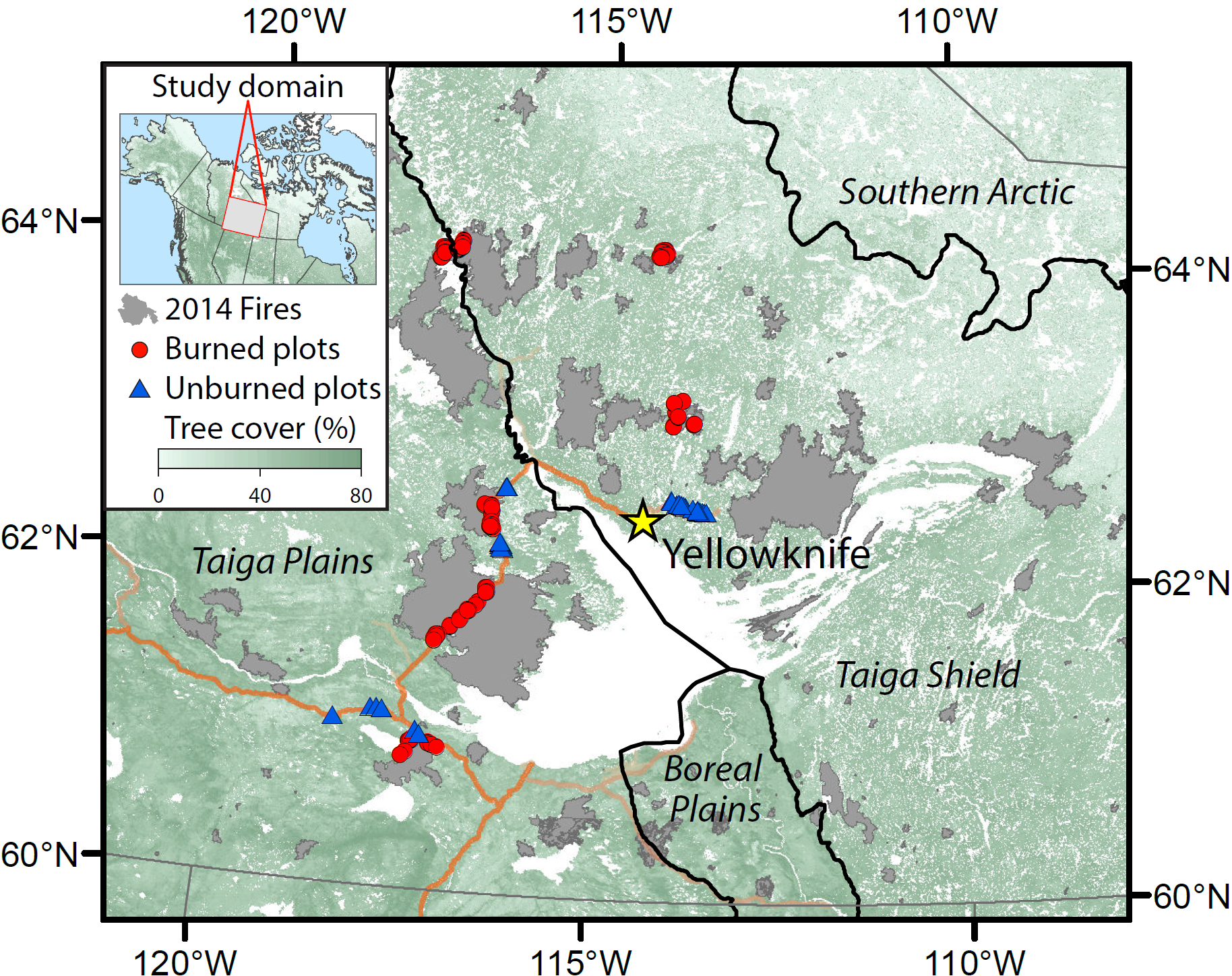
Figure 3. Map of study area.
Field Methods
Burned areas:
Field data from burned plots, including measurements necessary to calculate carbon emissions as well as properties that influence combustion, were collected between June and August of 2015 in seven spatially independent burn scars, four in the Taiga Plains ecozone and three in the Taiga Shield ecozone, which had burned between June and August 2014. Within each burn, random sampling points were identified based on stratum of conifer density identified by the Land Cover Map of Canada 2005, produced from 250-m Moderate Resolution Imaging Spectroradiometer (MODIS) imagery (Latifovic et al., 2004), date of burn (early, mid, late season), and whether a plot was a “reburn” based on fire history information. Where Forest Resource Inventory data were available the leading tree species (black spruce or jack pine) was also identified. For ease of access the random sampling points were constrained to be within 1-km of highways or lake shorelines. Three to 12 random points (‘A’ plots) were located within each conifer density stratum or leading tree species (black spruce or jack pine) for each burn. Moisture classes, based on topography-controlled drainage were assessed and adjusted for soil texture and presence of permafrost for each random point on a six-point scale, ranging from xeric to subhygric, using the method outlined by Johnstone et al., (2008). In addition, at least one, but usually two, other points ('B' and 'C' plots) were identified that were of a different moisture class and within 100-500 m of the random point. A site was defined as the combination of the random plot and these additional plots. A total of 211 burned plots nested within 78 randomly located sites were sampled (Walker et al., 2018).
Unburned areas:
In June of 2016, field work was conducted in three spatially independent areas of forest, two in the Taiga Plains and one in the Taiga Shield (Fig. 3), that had no history of fire since records began in the NWT, in 1965. The selection procedure for unburned plots was designed to ensure they best matched conditions at burned plots. For 36 randomly selected burned plots, 30-m unburned sampling locations were subset by those that had the same aspect quadrant (N, E, S, W, or flat), based on the Canadian Digital Elevation Model (CDEM, http://www.geobase.ca), and that had pre-fire tree cover (Hansen et al., 2013) within ± 2% of the burned plot. Plots were selected that most closely matched the slope of the given burned plot based on the CDEM (Walker et al., 2018).
At each plot we recorded latitude, longitude, and elevation with a GPS receiver, and slope and aspect with a clinometer and compass. Each plot consisted of two 30-m parallel transects that were 2-m apart. Transects ran due north.
Field measurements:
Soil measurements were made along both transects within each plot. In burned and unburned stands, soil organic layer (SOL) depth was measured every six m (10 points/plot). The top 15 cm of the SOL profile were collected to assess soil C in unburned plots or the entire residual SOL profile in burned plots, at five points per plot along one transect. An intact sample of the SOL of approximately 5-cm x 10-cm was collected using a serrated knife and pruners. Dimensions of each SOL sample were recorded in the field. Organic samples were immediately frozen until they could be processed in the lab. In addition to the ten SOL depth measurements, the SOL depth was measured near the base of ten trees per plot for burn depth calibrations. At these points, the SOL depth was measured as close to the tree as possible. In association with these points, the depth from the top of the green moss to the closest adventitious root was measured on 1-3 adventitious roots per tree in unburned stands, and the height from the highest adventitious root height (ARH) to the top of the residual SOL on 1-3 adventitious roots per tree in burned stands.
In each plot, the basal diameter of trees < 1.3 m tall that were originally rooted within a 2-m x 30-m belt transect was measured. Fallen trees that were killed by fire were included in this census. Tree combustion was assessed where each tree was ranked from 0 to 3; 0=none, alive and no biomass combusted; 1=low, only needles/leaves consumed; 2=moderate, all foliage and majority of fine branches combusted; 3=high, most of the aboveground canopy including foliage, branches, and bark combusted. To estimate stand age, five tree disks were collected in burned stands or five tree cores in unburned stands from each of the dominant tree species within a stand, either black spruce, jack pine, or both species.
Laboratory Methods
Soil bulk density and carbon (C) content in relation to depth was assessed from 507 samples from 137 monoliths collected in 36 unburned plots and 1076 samples from 345 monoliths obtained from 134 burned plots.
Tree disks and cores were processed using standard dendrochronology techniques (Cook et al.,1990) and tree rings were counted as an estimate of time since last fire (see Walker et al., 2018(b) for details).
Stem counts, diameter, measurements and published allometric equations (Lambert et al., 2005) were used to calculate tree density (number stems m-2), basal area (m2 ha-1), and aboveground biomass (kg dry matter m-2) of the total tree, bark, main branches, fine branches, and needles/leaves, for each tree species in each plot. Total tree biomass combusted was calculated per tree from the assigned combustion class and affected biomass components (foliage, branches, and bark). Individual tree estimates were summed and divided by the sample area to estimate pre-fire biomass and biomass combustion (kg dry matter m-2) per plot. A biomass C content of 50% was assumed.
The adventitious root method and calibrations described in Walker et al., (2018) was used to calculate depth of burn in black spruce dominated stands. Total depth of pre-fire SOL was then reconstructed by adding the ARH and the associated offset to the residual SOL depth. In jack pine dominated plots, where ARH measurements were not possible, depth of SOL combustion was assessed by subtracting the residual SOL from the unburned average SOL depth associated with each moisture category (see Walker et al., 2018 (b)).
Soil C content model development
Soil carbon content was modeled as a function of depth using soil monoliths from unburned and burned plots. For each soil monolith (n=534), the cumulative sums of carbon content by 5 cm depth increments (n=1518) were calculated starting from the surface, which was 0 cm in unburned plots, but was adjusted according to burn depth in burned plots. Monoliths from both burned and unburned plots were used to ensure that the full range in SOL depths was captured. Linear mixed effects models were fit with a hierarchical random effects structure of soil monolith nested within plot, nested within unburned area or burn scar. Separate models were fit for black spruce and jack pine dominated plots. The full models included covariates for depth, ecozone, and moisture category, and their first order interactions. Model reduction was completed through backward selection using likelihood ratio tests of the full model against the reduced models.
The models specific to each forest type were used to predict the carbon content (kg C m-2) of both combusted (based on burn depth) and residual SOL for 10 measurements per plot. Pre-fire SOL carbon pools were calculated by summing the residual and the combusted carbon pools, which were then averaged per plot. For subsequent analysis we used the measured residual SOL carbon pool from the 134 plots for which direct measurements were made and the predicted SOL carbon pool from the remaining 77 plots.
Calculated carbon combustion
Three measures of carbon combustion were calculated for each plot: 1) total carbon combusted as the sum of above and belowground C combustion, 2) proportion of pre-fire C combusted as total C divided by the total pre-fire carbon, and 3) proportional of total C attributed to the soil organic layer as belowground C combustion divided by total C. Plot attributes were examined associated with fuel and weather conditions on the day of burning (Table 3). Refer to Walker et al., 2018(b) for additional details.
Table 3. Covariates included in each of the candidate models to predict total carbon combusted, total carbon combusted relative to total pre-fire carbon, and the proportion of soil carbon combusted relative to total carbon combusted.
| Model | Variables |
|---|---|
| Null Model | None |
| M1: Plot-level attributes | Moisture class Elevation Stand age Latitude |
| M2: Pre-fire Stand Composition | Black spruce proportion Total above ground biomass |
| M3: Fire Attributes | Date of burn Fine Fuel Moisture Code Drought Moisture Code |
| M4: Plot-level attributes + Pre-fire Stand Composition | M1 + M2 |
| M5: Plot-level attributes + Fire Attributes | M1 + M3 |
| M6: Pre-fire Stand Composition + Fire Attributes | M2 + M3 |
| Full Model | M1 + M2 + M3 |
Spatial modeling
A model was derived using only covariates obtainable from geospatial layers that covered the entire spatial domain of interest. Initially, 71 spatial layers were considered that were associated with topography, permafrost condition, fire severity, tree cover, peatland cover, date of burn, fire weather, tree species biomass and percent cover, and soil properties. Values for each plot were extracted using weighted averages of relevant pixels covering our 2 x 30-m transects. Model reduction was completed through backward stepwise election using likelihood ratio tests of the full model against the reduced models. For the minimum adequate model, residual plots were examined to test for heteroscedasticity and non-normality. For prediction purposes, the model’s expected values were back-transformed from a log to a natural scale assuming a log-normal distribution (i.e., accounting for bias in the mean estimate), resulting in a multiplicative nonlinear regression model.
The final model was used to estimate total C emissions at 30-m resolution across all fires in the 2014 NWT fire complex. First, burned pixels were estimated such that a pixel was defined as burned if it was defined as land according to the Sexton et al. (2013) tree cover database, was contained in the Canadian National Fire Database (Canadian Forest Service, 2017), and had a dNBR value of at least 0.1. However, not all land pixels had valid dNBR values, and an estimated total burned area was provided for the 2014 NWT complex by summing the area of pixels defined above with those that were not covered by our dNBR dataset but had valid land pixels within the fire perimeters, multiplied by the fraction of pixels that exceeded our 0.1 dNBR threshold within fire scars.
To apply the model across all fire perimeters, final model covariates were re-gridded to a common 30-m grid and Canadian Albers Equal Area Conic projection (bilinear interpolation for datasets coarser than 30-m and nearest neighbor for datasets 30-m or finer), defined by 29 tiles within the ABoVE 30-m reference grid (Figure 2). For consistency, the regression model was re-run with these downscaled covariates. The regression model was then applied to burned pixels defined by a threshold of Landsat-derived differenced Normalized Burn Ratio (dNBR) within fire perimeters. To limit unreasonably high combustion estimates, a maximum cap was applied on emissions of 1.2 times the maximum combustion observed at our field sites (9.26 kg C m-2. Note this only applied to 0.02% of pixels). To provide an estimate of total emissions from the 2014 NWT complex, the estimate of total emissions was scaled to the complex considering the fraction of burned area not covered by our model (4%), assuming mean combustion in the missing burned pixels (Walker et al., 2018).
Uncertainties
A Monte Carlo framework was adopted to quantify predictive uncertainty from measurement error in aboveground and belowground combustion, below, and landscape scaling. A total of 1,000 simulations were performed in which inputs varied within a distribution of influential parameters. A new spatial model was derived for each Monte Carlo simulation based on an updated estimate of total combustion in each plot.
Data Access
These data are available through the Oak Ridge National Laboratory (ORNL) Distributed Active Archive Center (DAAC).
ABoVE: Wildfire Carbon Emissions and Burned Plot Characteristics, NWT, CA, 2014-2016
Contact for Data Center Access Information:
- E-mail: uso@daac.ornl.gov
- Telephone: +1 (865) 241-3952
References
Beaudoin, A., P.Y. Bernier, L. Guindon, P. Villemaire, X.J. Guo, G. Stinson, T. Bergeron, S. Magnussen, and R.J. Hall. Mapping attributes of Canada’s forests at moderate resolution through kNN and MODIS imagery.Canadian Journal of Forest Research, 2014, 44(5): 521-532, https://doi.org/10.1139/cjfr-2013-0401
Canadian Forest Service (2017) National Fire Database - Agency FireData. Natural Resources Canada, Canadian Forest Service, Northern Forestry Centre, Edmonton, Alberta.
Cook, E.R. and L. Kairiukstis. (1990) ‘Methods of Dendrochronology: Applications in the Environmental Sciences.’ (Kluwer Academic Publishers: Dordrecht). doi 10.1007/978-94-015-7879-0
Hansen, M.C., P.V. Potapov, R. Moore, M. Hancher, S.A. Turubanova, A. Tyukavina, D. Thau, S.V. Stehman, S.J. Goetz, T.R. Loveland, A. Kommareddy, A. Egorov, L. Chini, C.O. Justice, and J.R.G. Townshend. 2013. High-Resolution Global Maps of 21st-Century Forest Cover Change. Science, 342, 850–853. https://doi.org/10.1126/science.1244693
Hengl T., J. Mendes de Jesus, G.B. Heuvelink, M. Ruiperez Gonzalez, M. Kilibarda, A. Blagotic, et al. 2017. SoilGrids250m: Global gridded soil information based on machine learning. PLoS One 12(2):e0169748. https://dx.doi.org/10.1371/journal.pone.0169748
Johnstone J.F., T.N. Hollingsworth, and F.S. Chapin III. (2008). A key for predicting postfire successional trajectories in black spruce stands of interior Alaska. General Technical Report - Pacific Northwest Research Station, USDA Forest Service, i + 37 pp.
Johnstone, J. and F. Chapin. 2006. Effects of soil burn severity on post-fire tree recruitment in boreal forest. Ecosystems, 9, 14–31. https://dx.doi.org/10.1007/s10021-004-0042-x
Latifovic, R., Z-L. Zhu, J. Cihlar, C. Giri, and I. Olthof. 2004. Land cover mapping of North and Central America—Global Land Cover 2000. Remote Sensing of Environment, 89, 116–127. https://doi.org/10.1016/j.rse.2003.11.002
Lambert, M-C., C-H. Ung, and F. Raulier. 2005. Canadian national tree aboveground biomass equations. Canadian Journal of Forest Research, 35, 1996–2018.https://doi.org/10.1139/x05-112
Sexton, J. O., X.-P. Song, M. Feng, P. Noojipady, A. Anand, C. Huang, C., D.-H. Kim, D.-H., K.M. Collins, S. Channan, C. DiMiceli, and J.G.R. Townshend. 2013. Global, 30-m resolution continuous fields of tree cover: Landsat-based rescaling of MODIS vegetation continuous fields with lidar-based estimates of error. International Journal of Digital Earth, 6 (5): 427–448. https://doi.org/10.1080/17538947.2013.786146
Walker X.J., J. Baltez, S. Cumming, N. Day, J. Johnstone, B. Rogers, K. Solvik, M. Turetsky, and M. Mack. (2018) Soil organic layer combustion in boreal black spruce and jack pine stands of the Northwest Territories, Canada. International Journal of Wildland Fire https://doi.org/10.1071/WF17095
Walker, X.J., B.M. Rogers, J.L. Baltzer, S.G. Cumming, N.J. Day, S.J. Goetz, J.F. Jpohnstone, E.A.G. Schuur, M.R. Turetsky, and M.C. mack. 2018(b). Cross-scale controls on carbon emissions from boreal forest megafires. Glob Change Biol. 2018;00:1–15. https://doi.org/10.1111/gcb.14287