Documentation Revision Date: 2025-06-06
Dataset Version: 1
Summary
This dataset contains 10 data files in comma-separated values (CSV) format.
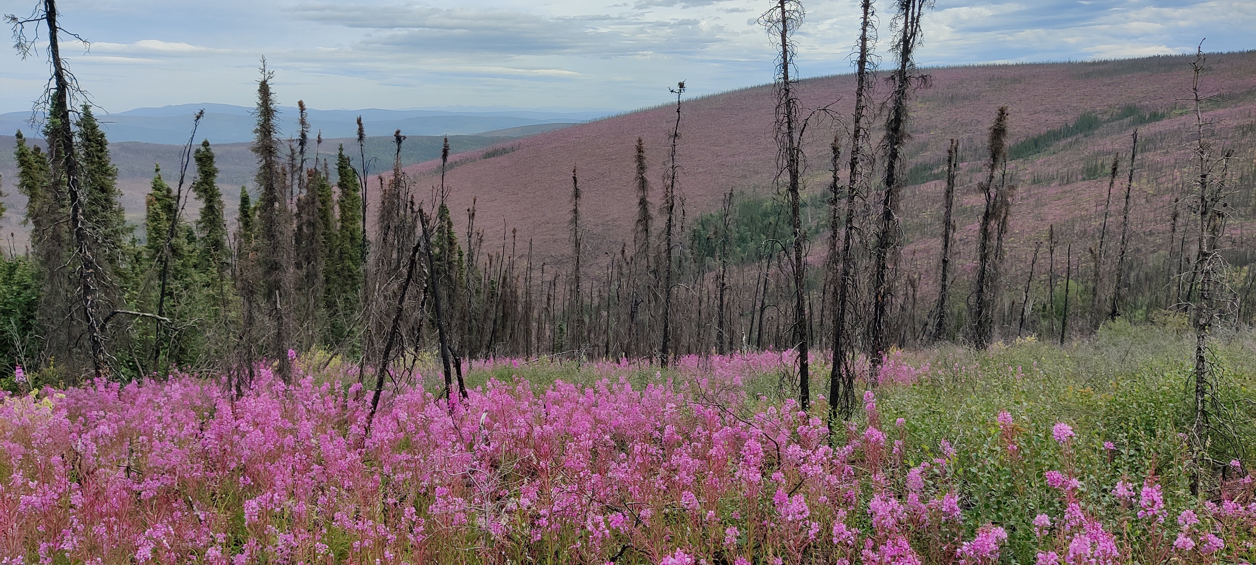
Figure 1. Severely burned and unburned conifer forest in Shovel Creek Watershed, August 2022, near Fairbanks, Alaska.
Citation
Huebner, D.C., C.S. Potter, and O. Alexander. 2025. ABoVE: Boreal Forest Resilience Study 2020-2022, Fairbanks AK. ORNL DAAC, Oak Ridge, Tennessee, USA. https://doi.org/10.3334/ORNLDAAC/2390
Table of Contents
- Dataset Overview
- Data Characteristics
- Application and Derivation
- Quality Assessment
- Data Acquisition, Materials, and Methods
- Data Access
- References
Dataset Overview
This dataset includes five metrics of forest resilience (recruitment, invasives, permafrost change, tree damage, and radial growth) at five recently burned forest sites (2010-2019) near Fairbanks, Alaska. The sites were imaged by the Airborne Visible InfraRed Imaging Spectrometer (AVIRIS-NG) in 2017 and 2022 during the Arctic-Boreal Vulnerability Experiment (ABoVE). Field measurements were conducted in 2021. Random forest (RF) vegetation classification models constructed from key hyperspectral bands were validated with ground-truthing (GT) of 44 measured plots and 45 geotagged plots. GT included stem densities, understory cover, soil characteristics, radial growth of 51 spruce trees from cores, and visual damage assays of 668 conifers and deciduous trees.
Project: Arctic-Boreal Vulnerability Experiment (ABoVE)
The Arctic-Boreal Vulnerability Experiment (ABoVE) is a NASA Terrestrial Ecology Program field campaign being conducted in Alaska and western Canada, for 8 to 10 years, starting in 2015. Research for ABoVE links field-based, process-level studies with geospatial data products derived from airborne and satellite sensors, providing a foundation for improving the analysis, and modeling capabilities needed to understand and predict ecosystem responses to, and societal implications of, climate change in the Arctic and Boreal regions.
Related Publications
Huebner, DC, CS Potter and Alexander. 2025. Assessing climate-wildfire effects on Alaskan boreal forest using ground-truth surveys and NASA airborne remote sensing. Journal of Vegetation Science, JVS-RES-06853. In review.
Huebner, D.C., and C.S. Potter CS. 2024. Comparisons of tree damage indicators in five NASA ABoVE forest sights near Fairbanks, Alaska [preprint]. BioRxiv. https://doi.org/10.1101/2024.07.10.602861
Acknowledgement
This research was supported by NASA through a contract with Oak Ridge Associated Universities and NASA Ames Research Center (STRIVES 20220017558).
Data Characteristics
Spatial Coverage: Sites near Fairbanks, Alaska
Temporal Coverage:
- AVIRIS-NG imagery: 2017-01-01 to 2022-12-31
- Field data: 2021-03-27 to 2021-09-13
Temporal Resolution: Field measurements from two consecutive summers: June-August 2021 and June-August 2022
Table 1. Site Information. For additional details, please see site_metadata.csv.
| Site | Latitude, Longitude (Decimal Degrees) | Year of AVIRIS dataset | Year of Ground Truth* | Sample size | ||
|---|---|---|---|---|---|---|
| Measured plots | Geotagged plots | Burned plots | ||||
| 2019 Shovel Creek Fire | 64.9747, -148.3124 | 2022 | 2021-22 | 13 | 10 | 8 |
| 2013 Skinny’s Road Fire | 64.7174, -148.6516 | 2017 | 2021-22 | 12 | 12 | 13 |
| 2012 Dry Creek Fire | 64.4703, -146.7230 | 2017 | 2021-22 | 1 | 4 | 0 |
| 2011 Moose Mountain Fire | 64.9591, -147.9275 | 2017 | 2021-22 | 13 | 8 | 4 |
| 2010 Willow Creek Fire | 64.6958, -148.3049 | 2017 | 2021-22 | 5 | 11 | 0 |
| Total | 44 | 45 | 25 | |||
*2021 field season: June 7 to August 31. 2022 field season: June 2 to August 16
Data file information
There are 10 data files in comma-separated values (*.csv) format in this dataset:
- AVIRIS_endmembers.csv
- Contains 89 polygons classified into 19 common endmembers using a subset of 29 AVIRIS bands at 5-m resolution and 5-nm bandwidth.
- GT_seedlings.csv
- Contains tree seedling densities measured in 45 circular plots (10.4-m radius) in 1 x 1-m grids and 5-m circular plots, upscaled to seedlings ha-1. MTBS classes from Monitoring Trends in Burn Severity.
- GT_understory.csv
- Contains understory vegetation measured in 45 circular plots identified using 6-letter species codes for boreal and arctic species. Please refer to Bonanza Creek LTER and/or Toolik Field Station herbarium for common species codes.
- GT_thermokarst.csv
- Contains thermokarst percent cover ha-1 and drunken tree stem densities were measured in 45 circular plots
- GT_soil_longform.csv
- Contains longform thaw depth (m), soil temperature C, and percent soil moisture were made in 10 data points x 3 transects in 45 circular plots.
- GT_upland_spruce_ring_widths.csv
- Contains longform ring width in mm and .001 mm by year for 18 spruce trees from lowland sites in the study area
- GT_lowland_spruce_ring_widths.csv
- Contains longform ring width in mm and .001 mm by year for 33 spruce trees from upland sites in the study area
- GT_z_scores_spruce.csv
- Contains distance from mean annual values for upland and lowland spruce ring width indices correlated to temperature and precipitation data by previous and current month of ring formation Temperature and precipitation data obtained from Bonanza Creek LTER (Van Cleave et al., 2021) and Fairbanks International Airport (NCEI, 2024).
- site_metadata.csv
- Contains location and study measurement characteristics from the five sites.
- tree_damage.csv
- Contains tree damage characteristics.
Table 2. Data Dictionary for AVIRIS_endmembers.csv. Note: # is used as a wildcard for variables containing ‘B#’ which reference AVIRIS-NG bands. Twenty-nine AVIRIS-NG bands were analyzed yielding 29 variables associated with each of these rows. Variables are labeled B1 through B29 in the data file.
| Variable | Units | Description |
|---|---|---|
| AVIRIS_transect | - | AVIRIS transect. ‘/’ is used a separator for rows associated with more than one transect |
| site | - | Site name. See Table 1 or site_metadata.csv for additional site details |
| Latitude | degrees north | Latitude in decimal degrees |
| Longitude | degrees east | Longitude in decimal degrees |
| class | - | Numeric identifier for ‘endmember’ categories |
| endmember | - | Dominant landcover type determined from classification models of average reflectance. Burn seveity codes: LB = light burn, MB = moderate burn, SB= severe burn |
| GT | - | Ground truthed: ‘YES’ indicates the polygon was ground-truthed via vegetation and soil measurements, ‘GEOTAG’ indicates that geotagged photos were taken of the site and vegetation class was determined from photographs with no additional cover and soil measurments made. |
| SEGMENTATION | - | Scale-merge-input bands algorithmused to group pixels based on similarity of pixels |
| REGION_ID | - | ID number of the segment |
| FX_AREA_m2 | m2 | Area of segment |
| pixels | 1 | Number of pixels in the segment |
| FX_LENGTH | m | Perimeter of segment |
| FX_COMPACT | 1 | Index that indicates compactness of segment: [Sqrt (4 * AREA / pi) / outer contour length] |
| FX_CONVEX | 1 | Index that measures convexity of the segment: [length of convex hull / LENGTH] |
| FX_SOLID | 1 | A shape index that compares the area of the polygon to the area of a convex hull surrounding the polygon. The solidity value for a convex polygon with no holes is 1.0, and the value for a concave polygon is less than 1.0. [AREA / area of convex hull] |
| FX_ROUND | 1 | A shape index that compares the area of the polygon to the square of the maximum diameter of the polygon. The maximum diameter is the length of the major axis of an oriented bounding box enclosing the polygon. The roundness value for a circle is 1, and the value for a square is 4 / pi. [4 * (AREA) / (pi * MAXAXISLEN2)] |
| FX_FORMFAC | 1 | A shape index that compares the area of the polygon to the square of the total perimeter. The form factor value of a circle is 1, and the value of a square is pi / 4. [(MAXAXISLEN = maximum axis length)] |
| FX_ELONG | 1 | A shape index that indicates the ratio of the major axis of the polygon to the minor axis of the polygon. The major and minor axes are derived from an oriented bounding box containing the polygon. The elongation value for a square is 1.0, and the value for a rectangle is greater than 1.0. [4 * pi * (AREA) / (total perimeter)2] |
| FX_RECT_FI | 1 | A shape index that indicates how well the shape is described by a rectangle. This attribute compares the area of the polygon to the area of the oriented bounding box enclosing the polygon. The rectangular fit value for a rectangle is 1.0, and the value for a non-rectangular shape is less than 1.0. [MAXAXISLEN / MINAXISLEN] |
| FX_MAIN_DI | degrees | The angle subtended by the major axis of the polygon and the x-axis in degrees. The main direction value ranges from 0 to 180 degrees. 90 degrees is North/South, and 0 to 180 degrees is ast/West. [AREA / (MAXAXISLEN * MINAXISLEN)] then convert radians to degrees |
| FX_MAJAXLN | degrees | The length of the major axis of an oriented bounding box enclosing the polygon. Values are map units of the pixel size. If the image is not georeferenced, then pixel units are reported. |
| FX_MINAXLN | map units | The length of the minor axis of an oriented bounding box enclosing the polygon. Values are map units of the pixel size. If the image is not georeferenced, then pixel units are reported. |
| FX_NUMHOLE | map units | The number of holes in the polygon. |
| FX_HOLESOL | 1 | The ratio of the total area of the polygon to the area of the outer contour of the polygon. The hole solid ratio value for a polygon with no holes is 1.0. |
| AVG_B# | 1 | Average value of the pixels comprising the band B#: [AREA / outer contour area] |
| STD_B# | radians | Standard deviation of the pixels comprising the band B# |
| X3SE_B# | nm | Three standard deviations of the wavelength of pixels comprising the band B# |
| MIN_B# | nm | Minimum value of the wavelength of pixels comprising the band B# |
| MAX_B# | nm | Maximum value of the pixels comprising the band B# |
| TXRAN_B# | nm | Average data range of the wavelength of pixels comprising the region inside the kernel of the band B#. A kernel is an array of pixels used to constrain an operation to a subset of pixels. |
| TXAVG_B# | nm | Average value of the wavelength of pixels comprising the region inside the kernel of the band B# |
| TXVAR_B# | nm | Average variance of the wavelength of pixels comprising the region inside the kernel of the band B# |
| TXENT_B# | nm | Average entropy value of the wavelength of pixels comprising the region inside the kernel of the band B# |
Table 3. Data dictionary for GT_lowland_spruce_ring_widths.csv and GT_upland_spruce_ring_widths_1.csv.
| Variable | Units | Description |
|---|---|---|
| Tree | - | Tree id consisting of polygon number followed by tree number (decimal) |
| Year | YYYY | Tree ring year |
| Ring_width_um | um | Tree ring width in micrometres (um) |
| Ring_width_mm | mm | Tree ring width in millimetres (mm) |
Table 4. Data dictionary for GT_seedlings.csv.
| Variable | Units | Description |
|---|---|---|
| plot | - | Unique plot name. Refer to Table 5 “site” column for naming convention. |
| site | - | Site name |
| latitude | degrees north | Latitude in decimal degrees |
| longitude | degrees east | Longitude in decimal degrees |
| habitat | - | Habitat type: ‘UPL’ for upland, ‘LL’ for lowland, ‘APL’ for alpine, and ‘ALP/UPL’ for alpine/upland |
| MTBS_burn_severity | - | Categories: Unburned, Light burn, Moderate burn, Severe burn |
| Burn_index | 1 | Range: 0 = unburned to 4 = severe burn |
| Endmember | - | Dominant landcover type determined from classification models of average reflectance. Burn severity codes: LB = light burn, MB = moderate burn, SB= severe burn |
| Year_of_Burn | YYYY | Year of last recorded burn, locations without a recorded burn are listed as ‘Unburned’ |
| Minimum_years_since_burn | y | Minimum number of years since last burn |
| Conifers_ha_1 | ha-1 | Number of conifers per hectare |
| Deciduous_trees_ha_1 | ha-1 | Number of deciduous trees per hectare |
| Live_trees_ha_1 | ha-1 | Number of live trees per hectare |
| Standing_dead_trees_ha_1 | ha-1 | Number f standing dead trees per hectare |
| Conifer_seedlings_ha_1 | ha-1 | Number of conifer seedlings per hectare |
| Deciduous_Seedlings_ha_1 | ha-1 | Number of deciduous seedlings per hectare |
| Total_Seedlings_ha_1 | ha-1 | Number of total seedlings per hectare |
| Tall_shrubs_ha_1 | ha-1 | Number of tall shrubs per hectare |
| Elevation | m | Elevation above sea level |
| Slope | degrees | Slope of sampling location in degrees |
| aspect | degrees | Aspect of sampling location in degrees |
| X_TK | 1 | Percent area of ground deformed by thermokarst (permafrost thaw/loss) |
| Drunken_trees_live_dead_ha_1 | ha-1 | Count per hectare of leaning trees due to permafrost thaw/loss under roots |
| logs_ha_1 | ha-1 | Number of logs per hectare |
Table 5. Data dictionary for GT_soil_longform.csv.
| Variable | Units | Description |
|---|---|---|
| year | YYYY | Year |
| month | - | Abbreviated month |
| DOY | d | Day of year |
| date | YYYY-MM-DD | Date of ground truth sampling |
| site | - | Letter codes refer to location in AVIRIS transect: DC (Dry Creek), MM (Moose Mountain), MD (Murphy Dome), ShovelCk (Shovel Creek), including borders/transition zones (ShovelCk/MD = Shovel Creek watershed near Murphy Dome/ Shovel Creek watershed near Moose Mountain ), SR (Skinnys Road). For ShovelCk, LB, MB SB, refer to burn class (Light burn, Moderate burn, Severe Burn). 4-5 digit numbers refer to polygon inside AVIRIS transect. 1-digit numbers refer to plot numbers sampled adjacent to but outside of AVIRIS transects. |
| habitat | - | Habitat type: ‘LL’ of lowland and ‘UPL’ for upland |
| Fire | - | Vegetation type (conifer, deciduous, mixed forest, shrubland, tundra, wetland) by habitat (LL = lowland, UPL = upland) by burn severity (UB = unburned, LB = light burn, SB = severe |
| Fire2 | - | Habitat type (lowland, upland) by burn severity (Unburned, Light, Moerate, Severe) |
| Fire3 | - | Burn severity code (UB = unburned, LB = light burn, MD= moderate burn, SB = severe burn) |
| Forest_type | - | Type of forest |
| endmember | - | Dominant landcover type determined from classification models of average reflectance. Burn severity codes: LB = light burn, MB = moderate burn, SB= severe burn |
| elevation | m | Elevation above sea level |
| slope | degrees | Slope of sampling location in degrees |
| aspect | degrees | Aspect of sampling location in degrees |
| radians | rad | Unit of angle inside circular sample plot |
| NORTHING_cos_radians | rad | Geographical coordinates inside circular sample plots |
| EASTING_SIN_radians | rad | Geographical coordinates inside circular sample plots |
| thaw_depth_m | m | Depth to ice from soil surface |
| soil_temp_C | degree C | Soil temperature at thaw depth |
| Percent_soil_moisture | 1 | Percent soil moisture |
Table 6. Data dictionary for GT_thermokarst.csv.
| Variable | Units | Description |
|---|---|---|
| Site | - | Described as in Table 5 |
| Endmember | - | Dominant landcover type determined from classification models of average reflectance. Burn severity codes: LB = light burn, MB = moderate burn, SB= severe burn |
| Burn_type | - | Burn severity categories: Unburned, Light, Moderate, Severe |
| Elevation | m | Elevation above sea level |
| Slope | degrees | Slope of sampling location in degrees |
| Aspect | degrees | Aspect of sampling location in degrees |
| Habitat | - | Habitat type: ‘UPL’ for upland, ‘LL’ for lowland, ‘APL’ for alpine, and ‘ALP/UPL’ for alpine/upland |
| Soil | - | Soil type: ‘Dry’, ‘Mesic’, or ‘Wet’ |
| Drunken_trees_ha_1 | ha-1 | Count per hectare of leaning trees due to permafrost thaw/loss under roots |
| Percent_thermokarst | 1 | Percent area of ground deformed by thermokarst (permafrost thaw/loss) |
Table 7. Data dictionary for GT_understory.csv. Please refer to Bonanza Creek LTER and/or Toolik Field Station herbarium for common species codes.
| Variable | Units | Description |
|---|---|---|
| Site | - | Described as in Tables 4, 5, 6. |
| Endmember | - | Dominant landcover type determined from classification models of average reflectance. Burn severity codes: LB = light burn, MB = moderate burn, SB= severe burn |
| Burn_type | - | Described as in Table 4 |
| Elevation | m | Elevation above sea level |
| Slope | degrees | Slope of sampling location in degrees |
| Aspect | degrees | Aspect of sampling location in degrees |
| Habitat | - | Habitat type: ‘UPL’ for upland, ‘LL’ for lowland, ‘APL’ for alpine, and ‘ALP/UPL’ for alpine/upland |
| Soil | - | Soil type: ‘Dry’, ‘Mesic’, or ‘Wet’ |
| Low_shrub | 1 | Percent cover of shrubs greater than 0.5 m height but less than 1 m heigh |
| Tallest_shrub_m | m | Height of tallest shrub in plot |
| Dwarf_deciduous_shrub | 1 | Percent cover of deciduous shrubs less than 0.5 m height |
| Dwarf_evergreen_shrub | 1 | Percent cover of evergreen shrubs less than 0.5 m height |
| Graminoid | 1 | Percent cover of grasses and sedges |
| Herbaceous_forb | 1 | Percent cover of herbaceous vascular species |
| Invasives | 1 | Percent cover of non-ntive plant species |
| Moss_liverworts | 1 | Percent cover of moss and liverworts |
| Percent_live_lichens | 1 | Percent cover of live lichens |
| Litter | 1 | Percent cover of unburned non-photosynthetic organic material (e.g., leaves, twigs) |
| Dominant_low_shrub_species | - | Dominant low shrub species |
| Char | 1 | Percent cover of charcoal |
| Bare_soil | 1 | Percent cover of bare soil |
| Dominant_dwarf_deciduous_shrub_pecies | - | Dominant dwarf deciduous shrub pecies |
| Dominant_dwarf_evergreen_shrub_species | - | Dominant dwarf evergreen shrub species |
| Dominant_graminoid_species | - | Dominant graminoid species |
| Dominant_forb_species | - | Dominant forb species |
| Dominant_invasive_species | - | Dominant invasive species |
| Dominant_moss_or_liverwort_species | - | Dominant moss or liverwort species |
| Dominant_lichen_species | - | Dominant lichen species |
Table 8. Data dictionary for GT_z_scores_spruce.csv. Temperature and precipitation data obtained from Bonanza Creek LTER (Van Cleave et al., 2021) and Fairbanks International Airport (NCEI, 2024).
| Variable | Units | Description |
|---|---|---|
| year | YYYY | Year of ring formation |
| UPL_z_scores | 1 | Z scores as departures from mean values of 0 for UPLAND growing trees (>200 m above sea level) |
| LL_z_scores | 1 | Z scores as departures from mean values of 0 for LOWLAND growing trees (< 200 m above sea level) |
| prev_Month_temp_z | 1 | Where prev Month temp is air temperature for each month in the year previous to tree ring formation. Months are represented by three-letter abbreviations. There are 12 of these variables. |
| Month_temp_z | 1 | Where Month temp is air temperature for each month in the year of tree ring formation. Months are represented by three-letter abbreviations. There are 12 of these variables. |
| prev_3Month_temp_z | 1 | Where prev 3month temp is air temperature for 3-month intervals in the year previous to tree ring formation. 3-month intervals are represented by one-letter abbreviations of sequential months. There are 10 of these variables. |
| prev_ND_curr_J_temp_z | 1 | Where prev ND represents November and December of the previous year of tree ring formation and curr J represents the current January n the year of tree ring formation. |
| 3Month_temp_z | 1 | Where 3month temp is air temperature for 3-month intervals in the current year of tree ring formation. 3-month intervals are represented by one-letter abbreviations of sequential months. There are 9 of these variables. |
| prev_ Month_prec_z | 1 | Where prev.Month prec is precipitation for each month in the year previous to tree ring formation. Three-letter abbreviations are used for each month. There are 12 of these variables. |
| Month_prec_z | 1 | Where Month prec is precipitation in the month of the current year of tree ring formation Three-letter abbreviations are used for each month. There are 12 of these variables. |
| prev_3month_prec_z | 1 | Where prev 3month prec is precipitation for 3-month intervals in the year previous to tree ring formation. 3-month intervals are represented by one-letter abbreviations of sequential months. There are 12 of these variables. |
| 3month_prec_z | 1 | Where prev 3month prec is precipitation for 3-month intervals in the year of tree ring formation. 3-month intervals are represented by one-letter abbreviations of sequential mnths. There are 12 of these variables. |
Table 9. Data dictionary for site_metadata.csv.
| Variable | Units | Description |
|---|---|---|
| Site | - | Site name |
| Latitude | degrees north | Latitude of site in decimal degrees |
| Longitude | degrees east | Longitude of site in decimal degrees |
| Fire_year | YYYY | Year fire occurred, or Unburned |
| AVIRIS_year | YYYY | Year AVIRIS transect was flown. 'NA' indicates site is outside of AVIRIS transect |
| GT_year | YYYY | Year site was ground-truthed |
| n_plots_measured | 1 | Number of plots measured |
| n_plots_geotagged | 1 | Number of plots geotagged |
| n_plots_burned | 1 | Number of plots burned |
Table 10. Data dictionary for tree_damage.csv.
| Variable | Units | Description |
|---|---|---|
| plot | - | Refer to Table 4 “plot” and Table 5 “site” for naming convention |
| site | - | Site name |
| habitat | - | Habitat type: ‘UPL’ for upland, ‘LL’ for lowland, ‘APL’ for alpine, and ‘ALP/UPL’ for alpine/upland |
| MTBS_burn_severity | - | Categories: Unburned, Light burn, Moderate burn, Severe burn |
| Burn_index | 1 | Range: 0 = unburned, 4 = severe burn |
| Endmember | - | Dominant landcover type determined from classification models of average reflectance. Burn severity codes: LB = light burn, MB = moderate burn, SB= severe burn |
| Year_of_Burn | YYYY | Year fire occurred, or Unburned |
| Minimum_years_since_burn | y | Number of years since burn; 100 years minimum if Unburned |
| Tree_ID | - | Unique ID for each tree in plot from 120 unless otherwise noted |
| Age_class | - | Age class: ‘Tree’ or ‘Seedling’ |
| Species | - | Tree species |
| dbh_cm | cm | Tree diameter at breast height |
| PFT | - | Plant functional type: ‘Conifer’ or ‘Deciduous’ |
| basal_area_m2 | m2 | Square area occupied by tree stems |
| Height_m | m | Tree height in meters |
| Leaf_color_50 | - | Leaf color |
| observed | - | Notes on condition of tree |
| Leaf_damage | 1 | Range: 0 = no damage to 5 = severe damage |
| Stem_damage | 1 | Range: 0 = no damage to 5 = severe damage |
| Browning_index | 1 | Range: 0 = no damage to 5 = severe damage |
| wilting | 1 | Range: 0 = no damage to 5 = severe damage |
| Average_tree_damage | 1 | Range: 0 = no damage to 5 = severe damage |
| Conifers_ha_1 | ha-1 | Conifers per hectare |
| Deciduous_trees_ha_1 | ha-1 | Deciduous trees per hectare |
| Live_trees_ha_1 | ha-1 | Live trees per hectare |
| Standing_dead_trees_ha_1 | ha-1 | Standing dead trees per hectare |
| Conifer_seedlings_ha_1 | ha-1 | Conifer seedlings per hectare |
| Deciduous_Seedlings_ha_1 | ha-1 | Deciduous seedlings per hectare |
| Total_Seedlings_ha_1 | ha-1 | Total seedlings per hectare |
| Elevation | m | Elevation above sea level |
| Slope | degrees | Slope of sampling location in degrees |
| aspect | degrees | Aspect of sampling location in degrees |
| radians | rad | Unit of angle inside circular sample plot |
| NORTHING_cos | rad | Geographical coordinates inside circular sample plots |
| EASTING_sin | rad | Geographical coordinates inside circular sample plots |
| Tall_shrubs_ha_1 | ha-1 | Tall shrubs per hectare |
| Percent_Moss | 1 | Percent cover of moss |
| Percent_Litter | 1 | Percent coer of unburned non-photosynthetic organic material (e.g., leaves, twigs) |
| Percent_Char | 1 | Percent cover of charcoal |
| Percent_Char_year_1 | yr-1 | Percent cover of charcoal divided by the number of years since the fire |
| d_Thaw | m | Change in thaw depth from early summer to late summer |
| d_Temp | degree C | Change in soil temperature from early summer to late summer |
| Max_thaw_depth_m | m | Depth to ice from soil surface |
| Max_soil_temp_C | degree C | Soil temperature at maximum thaw depth |
| Percent_soil_moisture | 1 | Percent soil moisture |
| Percent_TK | 1 | Percent area of ground deformed by thermokarst (permafrost thaw/loss) |
| Drunken_trees_live_dead_ha_1 | ha-1 | Count per hectare of leaning trees due to permafrost thaw/loss under roots |
| logs_ha_1 | ha-1 | Logs per hectare |
Application and Derivation
This is the first ground truth validated study of pre- and post-fire boreal forest near Fairbanks Alaska imaged with hyperspectral technology since Ustin and Xiao (2001).
Quality Assessment
A variety of tasks was performed to account for error and uncertainty. See Section 5 below.
AVIRIS-NG images were acquired by NASA aircraft in optimal conditions between June-August of 2017 and 2018 to ensure optimal condition of photosynthetic canopies. Flights were chosen on clear days to minimize presence of clouds.
Hyperspectral data: average reflectance values and indices (e.g., NDVI, non-photosynthetic carbon index, and water use efficiency index) were calculated and compared to the literature for initial analysis of greenness and forest health. Bands were selected to capture the normal range of pre- and post-succession vegetation characteristics of the area by leaf pigmentation and water content with a minimum of spectral overlap (high between-class variation, low within-class variation). Rulesets used to classify vegetation types were constructed with high between-class, low within-class spectral ranges to minimize uncertainty.
All ground-truthed measurements were conducted to ensure variables were randomly sampled and independent. Sites were selected to minimize edge effects and other unwanted effects (e.g., soil compaction from vehicles or hikers) while being accessible via short hikes from roads or trails. Field measurements were conducted a maximum of three times per measurement per visit using field instruments that were calibrated daily before use (as for soil temperature and moisture). Sites were visited a maximum of twice per season where appropriate to assess seasonal changes in soil characteristics, however, it was not possible to visit each site on the same date in each sample year, so some of the seasonal data on soils reflects inter-annual effects. Field measurements in circular plots were conducted in transects moving clockwise to minimize trampling of understory vegetation. All collected datapoints were plotted to assess data for distribution shape and outliers prior to further analysis. Mean values presented in the study included standard errors and/or 95% confidence intervals where appropriate to show the spread in the data to account for natural variation and ranges of uncertainty.
Data Acquisition, Materials, and Methods
Image processing and vegetation classification of study area
AVIRIS scenes were initially processed from 29 spectral bands across the VIS and NIR spectrum (416.9 -1283 nm) selected to identify average reflectance changes in chlorophyll and water content. Images were segmented into natural boundaries (polygons) using the 64-bit ENVI 5.5 software (Wolfe and Black, 2018) and spectrally analyzed for fire fuel loads and forest health (Huebner and Potter, 2024 preprint). Endmembers describing common interior vegetation classes were defined using machine learning. Supervised significance analysis of microarrays (SAM) determined the similarity between an image spectrum (from all undefined land covers) and a reference spectrum (representing a known plant species location) by computing the spectral angle between them and treating them as vectors in n-dimensional spectral space, where n is the number of spectral bands. For each reference spectrum chosen from an AVIRIS-NG image, ENVI computes each spectral angle in radians for every image pixel and determine its closest statistical match among all the angles in the reference plant species to generate new land cover map outputs. This allows a comparison of vegetation dynamics and ground surface changes across burned and unburned areas within AVIRIS-NG image footprints, most of which are inaccessible from roads and rivers. Using Python’s Scikit-learn library (Bac et al., 2021) of classification algorithms, the following were tested: decision trees, random forest (RF), naïve bayes, k-nearest neighbor, logistic regression, and support vector machine (SVM).
RF builds an ensemble of decision trees through sampling with replacement of independently selected variables for each tree. Each node of a tree is split by determining which variable creates the most homogeneity using Gini impurity. For classification, majority voting from each tree’s classification is used to generate an aggregated classification of the tested datapoint. For pre-GT model training, 80% of the datapoints were selected while the remaining 20% was used to test model performance. The pre-GT ruleset was built from a 9-band hyperspectral subset, derived from uncorrelated Stable Zone Unmixing that selects bands with high between-endmember/ low within-endmember variance and low correlation, after Tane et al. (2018). The same ruleset was applied across four AVIRIS scenes imaged in 2017-2018: the 2010 Willow Creek Fire, the 2011 Moose Mountain Fire, the 2012 Dry Creek Fire, and the 2013 Skinny’s Road Fire. For RF model 1, 12 endmembers describing typical upland (>200 m elevation) and lowland forest successional stages were used, and for RF model 2, two additional endmembers were added. Model accuracy was compared post-GT, and new models were constructed using local spectral ranges unique to each AVIRIS-NG scene (‘unique models’) to describe 19 endmembers verified in GT. Average reflectance was broadcasted in each endmember by 1%, 5%, and 10% margins until > 50% accuracy and overall classification was achieved.
Ground truth (GT) surveys
GT plots were surveyed June to August of 2021 and 2022, when leaves are green and fully expanded. 89 polygons inside the AVIRIS-NG scenes representing upland and lowland forest communities (average area 35,000 m2) were selected for GT; a subset of 44 polygons was used for plant and soil measurements. 25 polygons were assigned burn severity classes (light, moderate, severe, and unburned) from Alaska Monitoring Trends in Burn Severity (MTBS) overlay maps (Eidenshink et al., 2007). A high-precision GPS unit was supplied by NASA (Garmin Inc., Olathe, KS USA) to geolocate sampling plots inside polygons. Plant and soil measurements were conducted in circular plots (10.36 m fixed radius) after Andersen et al. (2011). Plots were spaced >50 m from roads to avoid edge effects. Plots were nested at three spatial scales for sampling efficiency: broad (10.36 m radius) for tree measurements; intermediate (5 m radius) for tall shrubs ha-1 (>1 m height), coarse woody debris, tree seedling counts ha-1, and percent area of thermokarst; and fine (1 m2) for understory measurements. Understory percent cover by species was averaged from four randomly placed 1 x 1 m grids inside each plot; grids were subdivided into 100 squares (optical cramming) following Viereck et al. (1992). Understory consisted of low shrubs <1 m height, dwarf evergreen and deciduous shrubs <0.5 m height, graminoids, herbaceous forbs, cryptogams, litter, bare soil, charcoal (‘char’), and invasive (non-native) plant species. Tree seedlings not counted in the 5-m radius plots, upscaled to densities ha-1 were included. Depth to permafrost, using a 1.2 m thaw probe, and soil temperature and percent soil moisture, using an AQUATERR T-350 sensor (AQUATERR, Costa Mesa, CA USA) were averaged from 30 measurements in each plot.
Inter-endmember variation of GT characteristics
To understand the relationship between endmembers and ground characteristics, a ANOVA of linear models was used for each variable explaining endmembers, including burn severity index; densities ha-1 of live and dead trees, shrubs, seedlings, and logs; canopy height (m); tree diameter at breast height (dbh, cm); tree basal area (m2); elevation (m); slope (%); aspect (degrees); percent cover of low and dwarf shrubs, cryptogams, forbs, bare soil, char, and invasives; tree damage averaged from leaf, stem, wilting and browning scores; and soil properties including active layer depth (m), percent moisture, and temperature °C. Fifteen variables with the best fit (R2Adj) describing endmember variation were selected and coefficient of variation (CV; Brown, 1998) was computed for each variable.
Tree and cover measurements
Average tree densities ha-1 were upscaled from tree and seedling counts per plot. Twenty randomly selected focal trees or seedlings per plot (309 conifer, 359 deciduous) were measured for height with a clinometer (Suunto, Vantaa, Finland) and diameter at breast height (DBH) with a tape measure. Focal trees were visually assessed for leaf and stem damage and canopy color per crown area (modified from Boucher and Mead, 2006) by assigning dominant crown color (green, yellow or brown) forr each tree. Using indices of 0 - 5 (0 = no change, 5 = severe change) average tree damage was calculated from: 1) leaf damage, 2) stem damage, 3) wilting, and 4) browning (non-photosynthetic tissue in the canopy) (Huebner and Potter, 2024 preprint).
Statistical analysis of GT
Statistical analyses were performed in R (R Core Team 2024) and JMP 16.1.0 software (JMP® SAS Institute; Jones and Sall, 2011). One-way ANOVA was used to compare burn severity effects (MTBS levels: light, moderate, severe, unburned) on forest productivity (stem density of tree seedlings and tall shrubs ha-1), thermokarst presence, and drunken trees ha-1. To understand interannual effects on soils, thaw depth, soil temperature, and soil moisture were averaged by study year using one-way ANOVA by vegetation and habitat (upland, lowland). To understand seasonal soil response to summer conditions, linear and quadratic regressions of soil temperature and moisture averages were compared by day of year between study years. R-squared values were used to quantify regression model fit.
Tree radial growth
Because conifers produce clearer ring boundaries than deciduous species, 1-2 cores per tree were harvested from 123 upland and lowland white spruce (Picea glauca) and black spruce (P. mariana) using a 5-mm increment borer. Trees with heartwood rot were excluded from radial growth analysis and given a stem damage score of 5 for the visual tree damage survey (Huebner and Potter, 2024 preprint). Intact cores of old-growth trees (33 upland, 18 lowland) were glued onto wooden bases, polished with 100 to 600 grit sandpaper and digitally photographed at >600 dpi. Ring widths were measured from high resolution images to 0.001 mm a minimum of two times per sample to minimize errors using CooRecorder 9.8.1 software and cross-dated using CDendro (Maxwell and Larsson, 2021). Common growth signal strength was determined from detrended ring widths (30-year cubic smoothing spline) using within-population growth synchrony statistics: 1st order autocorrelation; mean sgc/ssgc (synchronous growth changes/semi- synchronous growth changes); rbarwt/rbar.bt (within-tree growth correlation/between-tree growth correlation); and mean subsample synchrony strength (sss) using the R ‘dplR’ package (Bunn 2008; Bunn et al. 2022). Sgc/ssg replaces the Glk (Gleichaufigkeit) test, since Glk can be influenced by years when a series shows no growth change (Bunn et al., 2022). Sgc/ssg describes within-population growth similarity divided by a percentage of years where at least one tree in a population shows no change in growth (Visser, 2020). Sss is used in place of EPS (see Bunn et al., 2022 and Buras, 2017).
Three chronologies were compared for each population, controlling for within-population auto-correlation that can mask growth response to climate: 1) the standard chronology or bi-weight mean value of ring widths; 2) the residual chronology, i.e., pooled auto-regressive order from residuals of the standard chronology; and 3) the ARSTAN chronology, which reintroduces auto-correlation coefficients from pooled multivariate modelling (Cook, 1985). Growth change of each population was correlated to air temperature and precipitation records averaged from Fairbanks International Airport 1929-2022 (Menne et al., 2012; NCEI, 2024) and Bonanza Creek Experimental Forest 1989-2022 (Van Cleve et al., 2021) with missing values supplemented by CRU climate data from the same coordinates (Harris et al., 2020). Moving windows climate-growth correlations (35-year windows at 1-year intervals) were performed with the R ‘treeclim’ package (Zang and Biondi, 2015), which calculates Pearson’s correlation coefficients between annual tree growth and monthly air temperature and precipitation. To understand climate-growth relationships by season, departures from mean annual tree growth were regressed against regional temperature and precipitation anomalies as z-scores (the difference between each datapoint and the overall mean divided by the standard deviation). Seasons were classified in 3-month increments from January, February, and March of the previous growth year (Prev. JFM) through August, September, and October of the current year (ASO). Alaska-wide drought indexes from 2001 – 2022, collected by the National Drought Information System (NIDIS) as percent land area at five levels: D0 abnormally dry conditions, D1 moderate drought, D2 severe drought, D3 extreme drought, and D4 exceptional drought (Brewer et al. 2006), were used to calculate percent change from mean growth for each spruce population.
Data Access
These data are available through the Oak Ridge National Laboratory (ORNL) Distributed Active Archive Center (DAAC).
ABoVE: Boreal Forest Resilience Study 2020-2022, Fairbanks AK
Contact for Data Center Access Information:
- E-mail: uso@daac.ornl.gov
- Telephone: +1 (865) 241-3952
References
Bac, J., E.M. Mirkes, A.N. Gorban, I. Tyukin, and A. Zinovyev, A. 2021. Scikit-dimension: a python package for intrinsic dimension estimation. Entropy 23:368. https://doi.org/10.3390/e23101368
Brewer, M., T. Owen, R. Pulwarty and M. Svoboda. 2006. National Integrated Drought Information System (NIDIS): A Model for Interagency Climate Services Collaboration.
Brown, C.E. 1998. Coefficient of Variation. Applied Multivariate Statistics in Geohydrology and Related Sciences:155–157. https://doi.org/10.1007/978-3-642-80328-4_13
Bunn, A.G. 2008. A dendrochronology program library in R (dplR). Dendrochronologia 26:115–124. https://doi.org/10.1016/j.dendro.2008.01.002
Bunn A.G., M. Korpela, F. Biondi, F. Campelo, P. Mérian, F. Qeadan, C. ange, A. Buras, A. Cecile, M. Mudelsee, M. Schultz, D. Frank, R. Visser, E. Cook, and K. Anchukaitis. 2022. Package dplR: Dendrochronology Program Library in R. https://CRAN.R-project.org/package=dplR
Buras, A. 2017. A comment on the expressed population signal. Dendrochronologia 44:130–132. https://doi.org/10.1016/j.dendro.2017.03.005
Cook, ER. 1985. A Time Series Analysis Approach to Tree Ring Standardization. PhD thesis, The University of Arizona. https://ltrr.arizona.edu/sites/ltrr.arizona.edu/files/bibliodocs/CookER-Dissertation.pdf
Eidenshink, J., B. Schwind, K. Brewer, Z.-L. Zhu, B. Quayle, and S. Howard. 2007. A project for monitoring trends in burn severity. Fire Ecology 3:3–21. https://doi.org/10.4996/fireecology.0301003
Harris, I., T.J. Osborn, P. Jones, and D. Lister. 2020. Version 4 of the CRU TS monthly high-resolution gridded multivariate climate dataset. Scientific Data 7. https://doi.org/10.1038/s41597-020-0453-3
Huebner, DC, CS Potter and Alexander. 2025. Assessing climate-wildfire effects on Alaskan boreal forest using ground-truth surveys and NASA airborne remote sensing. Journal of Vegetation Science, JVS-RES-06853. In review.
Huebner, D.C., and C.S. Potter CS. 2024. Comparisons of tree damage indicators in five NASA ABoVE forest sights near Fairbanks, Alaska [preprint]. BioRxiv. https://www.biorxiv.org/content/10.1101/2024.07.10.602861v1
Jones, B., and J. Sall. 2011. JMP statistical discovery software. WIREs Computational Statistics 3:188–194. https://doi.org/10.1002/wics.162
Maxwell, R.S., and L.-A. Larsson. 2021. Measuring tree-ring widths using the CooRecorder software application. Dendrochronologia 67:125841. https://doi.org/10.1016/j.dendro.2021.125841
Menne, M.J., I. Durre, B. Korzeniewski, S. McNeill, K. Thomas, X. Yin, S. Anthony, R. Ray, R.S. Vose, B.E. Gleason, and T.G. Houston. 2012. Global Historical Climatology Network - Daily (GHCN-Daily), Version 3. NOAA National Centers for Environmental Information. http://doi.org/10.7289/V5D21VHZ. [Accessed 07132024].
National Centers for Environmental Information (NCEI). 2024. Daily Summaries Station Details: FAIRBANKS INTERNATIONAL AIRPORT, AK US, GHCND:USW00026411 | Climate Data Online (CDO) | National Climatic Data Center (NCDC). Climate Data Online (CDO). https://www.ncdc.noaa.gov/cdo-web/datasets/GHCND/stations/GHCND:USW00026411/detail
R Core Team. 2024. R: A Language and Environment for Statistical Computing. Vienna: R Foundation for Statistical Computing. https://cran.r-project.org/
Tane, Z., D. Roberts, S. Veraverbeke, Á. Casas, C. Ramirez, and S. Ustin. 2018. Evaluating endmember and band selection techniques for multiple endmember spectral mixture analysis using post-fire imaging spectroscopy. Remote Sensing 10:389. https://doi.org/10.3390/rs10030389
Ustin, S.L., and Q.F. Xiao. 2001. Mapping successional boreal forests in interior central Alaska. International Journal of Remote Sensing 22:1779–1797. https://doi.org/10.1080/01431160118269
Van Cleve, K., F.S. Chapin, R.W. Ruess, and M.C. Mack. 2021. Bonanza Creek LTER: Hourly Air Temperature and Precipitation Measurements (sample, min, max) at 50 cm and 150 cm from 1988 to Present in the Bonanza Creek Experimental Forest near Fairbanks, Alaska, University of Alaska Fairbanks. ver 24. Environmental Data Initiative. https://doi.org/10.6073/pasta/b0141ea271c759ab7c9afab0d8b728e9
Viereck L.A., N.R. Werdin-Pfisterer, P.C. Adams, and K. Yoshikawa. 2008. Effect of wildfire and fireline construction on the annual depth of thaw in a black spruce permafrost forest in interior Alaska-A 36-year record of recovery. In Proceedings of the Ninth International Conference on Permafrost, University of Alaska Fairbanks, Fairbanks, Alaska. 29:1845-1850. https://research.fs.usda.gov/treesearch/32468
Visser, R.M., 2020. On the similarity of tree-ring patterns: Assessing the influence of semi-synchronous growth changes on the Gleichläufigkeit for big tree-ring datasets. Archaeometry 63:204-215. ;https://doi.org/10.1111/arcm.12600
Wolfe, J.D., and S.R. Black. 2018. Hyperspectral analytics in ENVI. NV5 Geospatial Software. https://www.nv5geospatialsoftware.com/Portals/0/pdfs/Confirmation/Hyperspectral-Whitepaper.pdf
Zang, C., and F. Biondi. 2015. Treeclim: an R package for the numerical calibration of proxy-climate relationships. Ecography 38:431–436. https://doi.org/10.1111/ecog.01335