Documentation Revision Date: 2020-11-09
Dataset Version: 1
Summary
To facilitate analyses, the Landsat 5 Thematic Mapper and Landsat 7 Enhanced Thematic Mapper data were reprojected into the ABoVE standard Alber’s equal area projection (30-m grid) and were gridded into 180 x 180 km ABoVE standard B grid tiles (Loboda et al., 2019). This resulted in a total of 175 B grid tiles over the ABoVE core domain. Land cover classifications (10- and 15-class products) are provided for each year from 1984 to 2014 for each tile.
This dataset provides 350 files with landcover data in GeoTIFF (.tif) format which includes 175 files for the 15-class product and 175 files for the 10-class product. Each file is a 31-band GeoTIFF, with each band providing one year of data for the 1984-2014 period, where band 1 is year 1984, band 2 is 1985, and so on until band 31, which is 2014. The accuracy assessment data are provided in two comma-separated (.csv) data files.
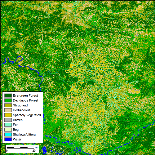
Figure 1. Land cover (10-class product) for the year 1984 in the ABoVE domain for analysis tile BH03V04. The pixel resolution is 30 m and a tile is 180 x 180 km. Refer to Figure 3 for the landcover in the same tile for the year 2014. (from ABoVE_LandCover_BH03V04.tif)
Citation
Wang, J.A., D. Sulla-Menashe, C.E. Woodcock, O. Sonnentag, R.F. Keeling, and M.A. Friedl. 2019. ABoVE: Landsat-derived Annual Dominant Land Cover Across ABoVE Core Domain, 1984-2014. ORNL DAAC, Oak Ridge, Tennessee, USA. https://doi.org/10.3334/ORNLDAAC/1691
Table of Contents
- Dataset Overview
- Data Characteristics
- Application and Derivation
- Quality Assessment
- Data Acquisition, Materials, and Methods
- Data Access
- References
Dataset Overview
This dataset provides two 30-m resolution time series products of annual land cover classifications over the Arctic Boreal Vulnerability Experiment (ABoVE) core domain for each year of the period 1984-2014. The data are the annual dominant plant functional type in a given 30-meter pixel derived from time series of Landsat surface reflectance, landcover training data mapped across the ABoVE domain using Random Forests modeling, with clustering and interpretation of field photography and very high resolution imagery to assign land cover classifications. One product has a 15-class land cover classification that breaks out forest and shrub types into several additional classes; the other product provides a simplified, 10-class approach. Classification accuracy assessment results are provided per year. Assessments were based on a probability-based random sample of reference data that supported statistically robust estimation of areas and uncertainties in mapped areas.
To facilitate analyses, the Landsat 5 Thematic Mapper and Landsat 7 Enhanced Thematic Mapper data were reprojected into the ABoVE standard Alber’s equal area projection (30-m grid) and were gridded into 180 x 180 km ABoVE standard B grid tiles (Loboda et al., 2019). This resulted in a total of 175 B grid tiles over the ABoVE core domain. Land cover classifications (10- and 15-class products) are provided for each year from 1984 to 2014 for each tile.
Project: Arctic-Boreal Vulnerability Experiment
The Arctic-Boreal Vulnerability Experiment (ABoVE) is a NASA Terrestrial Ecology Program field campaign taking place in Alaska and western Canada between 2016 and 2021. Climate change in the Arctic and Boreal region is unfolding faster than anywhere else on Earth, resulting in reduced Arctic sea ice, thawing of permafrost soils, decomposition of long-frozen organic matter, widespread changes to lakes, rivers, coastlines, and alterations of ecosystem structure and function. ABoVE seeks a better understanding of the vulnerability and resilience of ecosystems and society to this changing environment.
Related Publication
Wang, J. A., Sulla-Menashe, D., Woodcock, C. E., Sonnentag, O., Keeling, R. F., & Friedl, M. A. 2020. Extensive Land Cover Change Across Arctic-Boreal Northwestern North America from Disturbance and Climate Forcing. Global Change Biology 26, 807–822. https://doi.org/10.1111/gcb.14804
Related Dataset
Loboda, T.V., E.E. Hoy, and M.L. Carroll. 2019. ABoVE: Study Domain and Standard Reference Grids, Version 2. ORNL DAAC, Oak Ridge, Tennessee, USA. https://doi.org/10.3334/ORNLDAAC/1527
Acknowledgements
This research was funded by the NASA Terrestrial Ecology- Arctic and Boreal Vulnerability Experiment, grant numbers NNX17AE74G and NNX15AU63A and by the National Science Foundation (NSF) under grant number DGE-1247312..
Data Characteristics
Spatial Coverage: Alaska and Canada
ABoVE Reference Locations
Domain: Core ABoVE
The Landsat 5 Thematic Mapper and Landsat 7 Enhanced Thematic Mapper data were reprojected into the ABoVE standard Alber’s equal area projection (30-m grid) and were gridded into 180 x 180 km ABoVE standard B grid tiles (Loboda et al., 2019). This resulted in a total of 175 B grid tiles over the ABoVE core domain.
The two landcover classifications are provided for each tile for a total of 350 data files. The respective B grid tiles are identified in the filenames.
Spatial Resolution: 30 m
Temporal Coverage: 1984-01-01 to 2014-12-31
Study Area: (all latitudes and longitudes given in decimal degrees)
| Site (Region) | Westernmost Longitude | Easternmost Longitude | Northernmost Latitude | Southernmost Latitude |
|---|---|---|---|---|
| ABoVE domain: Alaska and Canada | -170.0058 | -98.97401389 | 76.225675 | 50.25900556 |
Data File Information
This dataset provides 350 files with landcover data in GeoTIFF (.tif) format which includes 175 files for the 15-class product and 175 files for the 10-class product. Each file is a 31-band GeoTIFF, with each band providing one year of data for the 1984-2014 period, where band 1 is year 1984, band 2 is 1985, and so on until band 31, which is 2014. The data values in each band represent the annual dominant plant functional type class (1-15 or 1-10; definitions in Table 2 & 3 below) in each 30-m pixel. The respective B grid tiles are identified in the filenames.
Land cover class accuracy assessment data are provided in two comma-separated (.csv) data files.
User Note: Using the ABoVE Standard Reference Grid System
As described, the Landsat data were reprojected into the ABoVE standard Alber’s equal area projection (30-m grid) and were then gridded into 180 x 180 km ABoVE standard B grid tiles. Each of the resulting data filenames includes the respective B grid tile coordinates (BhXXvZZ).
If a user wants to select landcover data files (B grid tiles) based on a defined bounding box, they can identify the respective ABoVE standard B grid tiles based on location by using the shapefiles provided in the related dataset (Loboda et al., 2019; https://doi.org/10.3334/ORNLDAAC/1527).
Table 1. File names and descriptions
| File names | Descriptions |
|---|---|
| ABoVE_LandCover_BhXXvZZ.tif |
Annual landcover classification of 15 plant functional types. The data provide the dominant plant functional type class for a given 30-m pixel in the identified ABoVE B grid tile (BhXXvZZ). Where XX is the horizontal ABoVE tile location and ZZ is the vertical ABoVE tile location for the respective B grid. |
| ABoVE_LandCover_Simplified_BhXXvZZ.tif |
Annual landcover classification of 10 plant functional types. The data provide the dominant plant functional type class for a given 30-m pixel in the identified ABoVE grid tile (BhXXvZZ). Where XX is the horizontal ABoVE tile location and ZZ is the vertical ABoVE tile location for the respective B grid. |
| accuracy_assess_1984-2014.csv | Classification accuracy assessment results (for the simplified 10-class version) for each year provided as error matrices. The columns indicate reference data and the rows indicate the classification. Refer to Table 4 for example data. |
| accuracy_summary_1984-2014.csv | Provides the producer's accuracy (inverse of error rate of omission), the user's accuracy (inverse of error rate of commission) for each class, as well as the overall accuracy for each year. |
GeoTIFF Data Descriptions
Two different land cover classifications are provided to describe the dominant plant functional type at a given pixel: 1) a classification with 15 different classes that breaks out forest and shrub types into several additional classes, and 2) a simplified approach with 10 different classes where forest and shrub types are aggregated.
File properties:
Bands: 31
No Data Value: 255
EPSG: 102001
Resolution: 30 m
Number rows x columns: 6,000 x 6,000
Missing values primarily occur as part of the ocean mask or for screened permanent snow/ice pixels.
Table 2. Land cover classes in the 15-class approach
| ID | Label | Description |
|---|---|---|
| 1 | Evergreen Forest | Area dominated by tall woody vegetation (> 3m tall) and over 60% canopy coverage with primarily (>75%) evergreen phenological habit (canopy maintains green foliage year-round). |
| 2 | Deciduous Forest | Area dominated by tall woody vegetation (> 3m tall) and over 60% canopy coverage with primarily (>75%) deciduous phenological habit (annual cycle of leaf-on and leaf-off periods). |
| 3 | Mixed Forest | Area dominated by tall woody vegetation (> 3m tall) and over 60% canopy coverage with neither forest type (deciduous or evergreen) exceeding over 60% of the area. |
| 4 | Woodland | Area dominated by tall woody vegetation (> 3m tall) with between 30-60% canopy coverage. Frequently co-exists with peatlands and typically, but not always, evergreen in phenological habit. |
| 5 | Low Shrub | Area dominated by dense hemi-prostrate to low-erect shrubs (5-30cm in height) with >60% area coverage. Analogous to "prostrate dwarf-shrub" and primarily occurring in tundra areas. |
| 6 | Tall Shrub | Area dominated by woody vegetation between 50cm and 3m tall and shrub canopy coverage >60% coverage. Typically, but not always, deciduous phenological habit. |
| 7 | Open Shrubs | Area with woody vegetation less than 3m tall and between 30-60% canopy coverage. Shrubs typically underlain by herbaceous or barren land cover. |
| 8 | Herbaceous | Area dominated by herbaceous land cover greater than 60% land cover and tree/shrub cover less than 10%. |
| 9 | Tussock Tundra | Tundra-specific herbaceous land dominated by Eriophorum vaginatum and other tussock-forming herbaceous species, coverage over 60%. |
| 10 | Sparsely Vegetated | 10-30% canopy coverage, any vegetation but typically herbaceous/bryophyte, with rock underneath |
| 11 | Fen | Hydrologically connected, sedge/grass dominated wetland |
| 12 | Bog | Ombrotrophic, peat and shrub dominated wetland |
| 13 | Shallows/littoral | Lakes <1m deep with some vegetation or shoreline mixed with water/land |
| 14 | Barren | <10% vegetation, mostly rock |
| 15 | Water | Oceans, lakes, and rivers, either salt-water or freshwater. |
Table 3. Land cover classes in the 10-class approach
| ID | Label | Combines the following classes from the 15-class approach | Combines the following labels: |
|---|---|---|---|
| 1 | Evergreen Forest | 1,4 | Evergreen Forest, Woodland |
| 2 | Deciduous Forest | 2,3 | Deciduous Forest, Mixed Forest |
| 3 | Shrubland | 5,6,7 | Low Shrub, Tall Shrub, Open Shrub |
| 4 | Herbaceous | 8,9 | Herbaceous, Tussock Tundra |
| 5 | Sparsely Vegetated | 10 | Sparsely Vegetated |
| 6 | Barren | 14 | Barren |
| 7 | Fen | 11 | Fen |
| 8 | Bog | 12 | Bog |
| 9 | Shallows/Littoral | 13 | Shallows/Littoral |
| 10 | Water | 15 | Water |
Accuracy assessment
File: accuracy_assess_1984-2014.csv
This file provides error matrices for classification accuracy assessment results by year, for the years 1984-2014 for the 10-class products. The results for the year 2014 are provided as an example. Reference data are indicated in columns; mapped classification data are in indicated rows. In the error matrix, correct classifications are shown along the diagonal and erroneous classifications are shown in the other cells. Refer to Table 3 for the landcover definitions.
Table 4. 10-class classification accuracy assessment for the year 2014.
| year | landcover | evergreen_forest | deciduous_forest | shrub | herb | sparse_veg | barren | fen | bog | shallows | water |
|---|---|---|---|---|---|---|---|---|---|---|---|
| 2014 | Everg. F | 223 | 9 | 19 | 9 | 5 | 9 | 10 | 2 | 7 | 3 |
| 2014 | Decid. F | 5 | 119 | 7 | 1 | 0 | 0 | 4 | 0 | 2 | 0 |
| 2014 | Shrub | 9 | 14 | 161 | 20 | 2 | 2 | 11 | 0 | 0 | 2 |
| 2014 | Herb | 0 | 1 | 11 | 93 | 4 | 1 | 3 | 0 | 1 | 3 |
| 2014 | Sparse Veg | 2 | 0 | 10 | 16 | 108 | 1 | 2 | 2 | 1 | 0 |
| 2014 | Barren | 0 | 2 | 3 | 6 | 8 | 52 | 2 | 4 | 1 | 4 |
| 2014 | Fen | 4 | 9 | 18 | 6 | 2 | 0 | 61 | 1 | 2 | 1 |
| 2014 | Bog | 5 | 0 | 0 | 0 | 0 | 0 | 2 | 39 | 0 | 0 |
| 2014 | Shallows | 2 | 0 | 0 | 4 | 3 | 0 | 1 | 0 | 30 | 2 |
| 2014 | Water | 1 | 1 | 4 | 1 | 4 | 2 | 0 | 0 | 9 | 69 |
File: accuracy_summary_1984-2014.csv
This file provides the producer’s classification accuracy (inverse of error rate of omission), user’s classification accuracy (inverse of error rate of commission), and overall classification accuracy for each class in the 10-class products for each year.
Table 5. Example data for the years 2014 and 2013.
| year | accuracy | evergreen_forest | deciduous_forest | shrub | herb | sparse_veg | barren | fen | bog | shallows | water |
|---|---|---|---|---|---|---|---|---|---|---|---|
| 2014 | prodAcc | 0.8884 | 0.7677 | 0.691 | 0.5962 | 0.7941 | 0.7761 | 0.6354 | 0.8125 | 0.566 | 0.8214 |
| 2014 | userAcc | 0.7534 | 0.8623 | 0.7285 | 0.7949 | 0.7606 | 0.6341 | 0.5865 | 0.8478 | 0.7143 | 0.7582 |
| 2014 | overAcc | 0.7467 | 0.7467 | 0.7467 | 0.7467 | 0.7467 | 0.7467 | 0.7467 | 0.7467 | 0.7467 | 0.7467 |
| 2013 | prodAcc | 0.8889 | 0.8125 | 0.7161 | 0.6562 | 0.8519 | 0.9155 | 0.6771 | 0.8776 | 0.6481 | 0.9059 |
| 2013 | userAcc | 0.8116 | 0.8904 | 0.7445 | 0.8268 | 0.7468 | 0.8125 | 0.619 | 0.86 | 0.7778 | 0.875 |
| 2013 | overAcc | 0.792 | 0.792 | 0.792 | 0.792 | 0.792 | 0.792 | 0.792 | 0.792 | 0.792 | 0.792 |
Application and Derivation
The data provide information on plant functional types in Arctic and Boreal biomes over a 31-year period which could help to quantify the loss, regrowth, and transitions between evergreen and deciduous tree species in the boreal forest biome at large spatial scales. See Wang et al (2019) for analysis details.
Quality Assessment
Two files are included that characterize the year by year accuracy for the simplified land cover classes across all years.
Following established practices for the assessment of remotely sensed land cover maps, the accuracy of the simplified land cover was assessed over each year by drawing a stratified random sample and creating a reference time series of land cover data for each site by visually interpreting very high-resolution imagery, field photography (geolocated photos provided by Kevin Turner (for the Old Crow Flats), Isla Myers-Smith (for Qikiqtaruk-Herschel Island), and Brendan Rogers, and time series of Landsat reflectance data (Olofsson et al., 2014). In reality, these data were stratified across a design intended to assess the accuracy of change detection. These reference data were adapted to year by year analyses and re-estimated year by year variances (Stehman, 2014). Table 6 provides an accuracy summary across all 31 years.
Table 6. Accuracy summary means
Producer’s accuracy refers to the inverse of error rate of omission, the user’s accuracy refers to the inverse of error rate of commission for each class. The overall accuracy for each year is also provided.
| accuracy | evergreen_forest | deciduous_forest | shrub | herb | sparse_veg | barren | fen | bog | shallows | water |
|---|---|---|---|---|---|---|---|---|---|---|
| Producer's Acc | 0.8891 | 0.7506 | 0.6949 | 0.6485 | 0.8096 | 0.8558 | 0.6418 | 0.8854 | 0.6567 | 0.8908 |
| User's Acc | 0.8266 | 0.881 | 0.6893 | 0.7882 | 0.7026 | 0.7902 | 0.6128 | 0.8586 | 0.7575 | 0.8883 |
| Overall Acc | 0.7735 | 0.7735 | 0.7735 | 0.7735 | 0.7735 | 0.7735 | 0.7735 | 0.7735 | 0.7735 | 0.7735 |
The land cover data does not correct for short-term changes in climate that may impact the spectral appearance of certain areas. For example, droughts may result in wetlands appearing drier, and subsequently being briefly classified as shrubs. Caution is advised when utilizing the wetland data for this reason (Wang et al., 2019).
Data Acquisition, Materials, and Methods
Study area
The study region included the core domain of NASA’s ABoVE project which includes the majority of Alaska and northwestern Canada and covers 4.67 x 10⁶ km2. To facilitate analyses, the Landsat 5 Thematic Mapper and Landsat 7 Enhanced Thematic Mapper data were reprojected into the ABoVE standard Alber’s equal area projection (30-m grid) and were gridded into 180 x 180 km ABoVE standard B grid tiles (Loboda et al., 2019). This resulted in a total of 175 B grid tiles over the ABoVE core domain.
The area mapped was defined by an ocean-land mask that was adopted from the 10-m ocean mask from Natural Earth data repository and manually edited to closely fit the Arctic coastline in our region (Wang et al., 2019).
Data processing
The primary source of data for land cover and disturbance mapping was time series of surface reflectance and brightness temperature from Landsat 5 and Landsat 7 retrieved from the ABoVE Science Cloud, covering the years 1984 to 2014. The Fmask algorithm was used to pre-process the Landsat image time series at each site to remove ephemeral contamination from clouds, snow, ice, cloud shadow, and other atmospheric effects that were not screened by the USGS (Zhu and Woodcock, 2012).
Disturbance detection and data modeling using CCDC
The minimum mapping unit and unit of analysis were 30-meter Landsat pixels within the ABoVE tiling system. For each pixel, the Change Detection and Classification (CCDC) algorithm (Zhu and Woodcock, 2014) was used to detect statistical breaks in time series of surface reflectance data. These breaks are hypothesized to represent land cover changes and the time segments intervening the breaks are assumed to be of stable land cover. The CCDC synthetic data was used to calculate a suite of surface reflectance metrics across bands and seasons to characterize the spectral-seasonal behavior of each time segment (e.g. spring versus summer values or annual amplitude for each band). In addition, several spectral indices were calculated as input features and the seasonal metrics were applied to them as well.
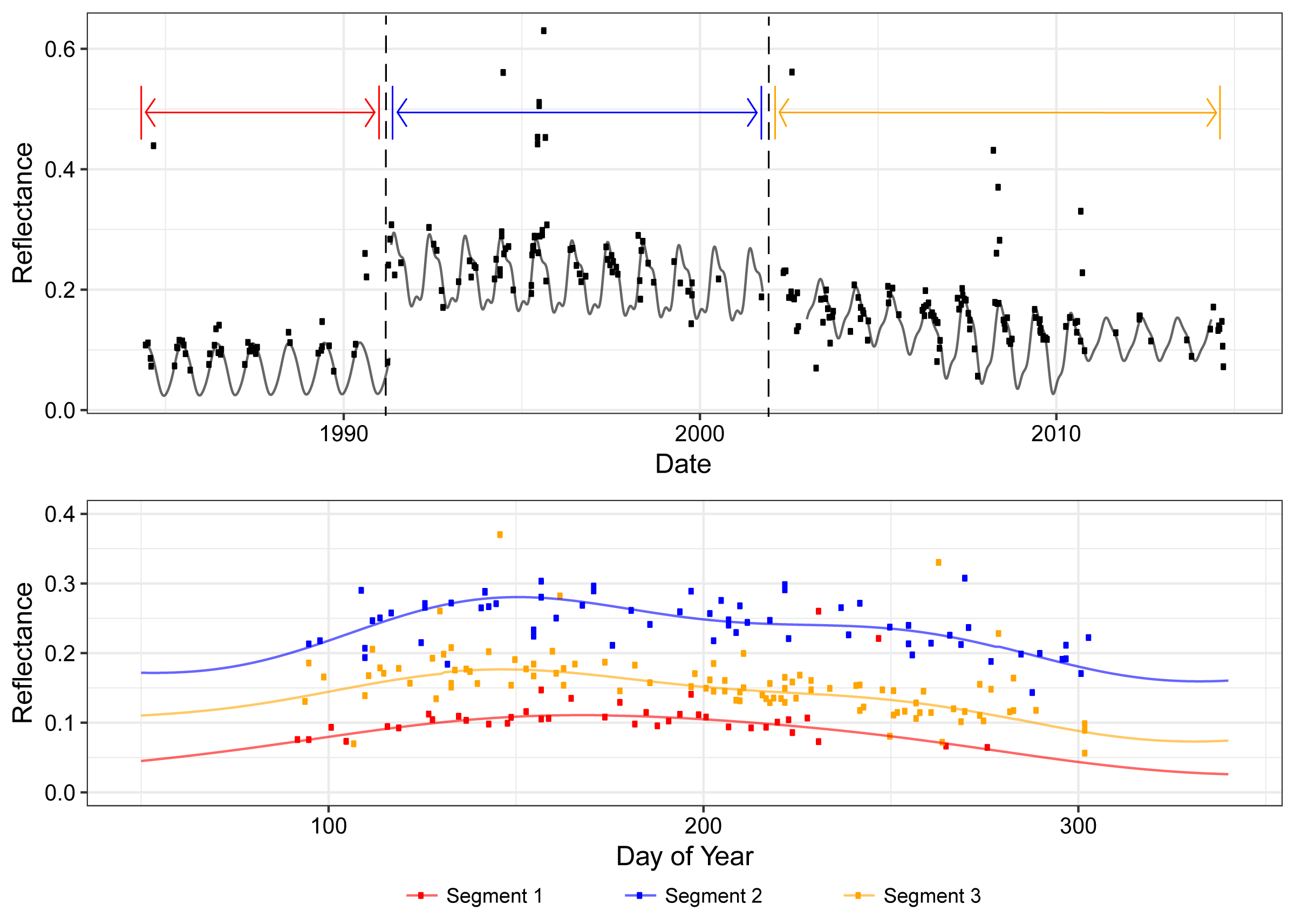
Figure 2. Example of time series and disturbance detection for one Landsat band and one pixel using the Continuous Change Detection and Classification (CCDC) algorithm. In this example, surface reflectance for Landsat band 5 (shortwave-infrared) is shown. Top panel: points are time series of observations reflectance, grey lines are fitted harmonic models, dashed vertical lines are the approximate timing of breaks in land cover, and colored horizontal lines and arrows indicate between-break time segments of stable land cover. CCDC detects and removes outliers in its model fits. Bottom panel: characteristic seasonal cycle of the color-coded time segments indicated in the top panel. Colored points indicate observations falling within the correspondingly colored time segments and lines indicate the harmonic model fit across those values, averaged across all years within the time segment.
Training and validating the land cover mapping algorithms
Training sites were generated across all ABoVE tiles via stratified random sampling (up to 10 per class in each tile) from existing land cover maps for Alaska and Canada circa 2000 (Jin et al., 2017; Wulder et al., 2008), ensuring coverage across a range of climatic conditions, spectral feature space, and ecosystem types. In total, the training data set included 15,628 sampled from the Canadian and Alaskan land cover datasets, 1,531 sites from the 10-m Scotty Creek land cover map (Chasmer et al., 2014), 970 sites from the Toolik Lake tundra vegetation map (Greaves et al., 2017, unpublished dissertation-data provided by personal communication), and 1,553 sites from field photographs for a total of 19,682 training sites (Wang et al., 2019).
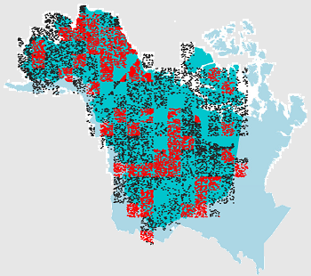
Figure 3. Points represent locations that were included in the clustering algorithm that was used to define the land cover legend and explore the spectral-temporal space within the ABR. Darker blue color indicates the ABoVE Core Study Domain (used for this study), while the lighter blue indicates the ABoVE Extended Study Domain (outside the scope of this study). Red points indicate sites were manually labelled by visual interpretation of very high-resolution imagery or field photographs. Black points were not manually labelled but were included in the clustering and the training data for the Random Forest algorithm (Wang et al., 2019).
Landcover class development
The training site data were clustered using a tree-based clustering method combining the R package treeClust (Buttrey and Whittaker, 2015). Each time segment was defined by a specific statistical cluster and mapped across the domain using Random Forest (Breiman, 2001). Each time segment was defined by a specific statistical cluster and mapped. The clusters were assigned meaningful land cover labels by visually interpreting a large sample (n = 10,136) of very high-resolution imagery (copyright DigitalGlobe), derived from IKONOS, Geo-Eye, QuickBird, Worldview-2, and Worldview-3, field photographs, and existing higher-resolution land cover maps (Chasmer et al., 2014; Greaves et al., 2017, unpublished dissertation-data provided by personal communication), as well as the Landsat surface reflectance time series. The clusters were cross-walked to land cover based on the interpretation of a set of land cover characteristics observed in these sources.
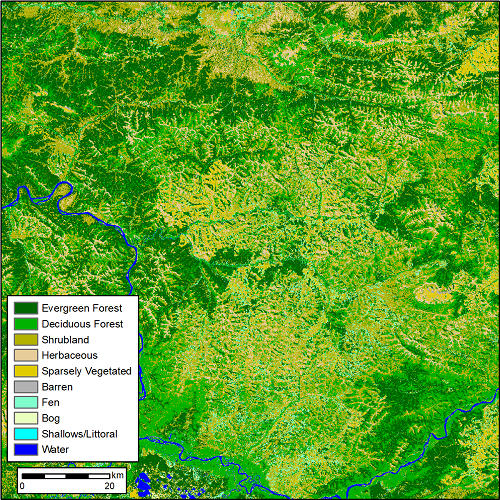
Figure 4. Land cover (10-class product) for the year 2014 in the ABoVE domain for analysis tile BH03V04. The pixel resolution is 30 m and a tile is 180 x 180 km. Refer to Figure 1 for the landcover in the same tile for the year 1984. (ABoVE_LandCover_BH03V04.tif)
Several post-processing steps resolved certain artifacts, including the removal of spurious land cover changes and the reduction of certain misclassifications. Once clusters have been reassigned to meaningful land covers, per-pixel series of time segments were analyzed and consecutive time segments with the same land cover label (but possibly differing clusters) were merged into single time segments of the same land cover. Additionally, time segments were extended forward or backward in time to cover time periods that had no CCDC output within a pixel. Therefore, missing data should only exist where Fmask identified 100% snow and ice or outside the ocean-land mask. Spurious classifications of water classes in mountainous regions were identified by comparing them with the slope of the pixel, derived from ASTER elevation data, and existing annual Landsat-based maps of global surface water status (Pekel et al., 2016). Those pixels that were mapped as water but had non-zero slope and were not classified as water by Pekel et al. 2016, were set to their second most likely class after water, using the Random Forest probabilities (Wang et al., 2019).
Data Access
These data are available through the Oak Ridge National Laboratory (ORNL) Distributed Active Archive Center (DAAC).
ABoVE: Landsat-derived Annual Dominant Land Cover Across ABoVE Core Domain, 1984-2014
Contact for Data Center Access Information:
- E-mail: uso@daac.ornl.gov
- Telephone: +1 (865) 241-3952
References
Breiman, L. Machine Learning (2001) 45:5. https://doi.org/10.1023/A:1010933404324
Buttrey, S.E., Whitaker, L.R., 2015. treeClust: An R package for tree-based clustering dissimilarities. The R Journal (2015) 7:2, pages 227-236
Chasmer, L., Hopkinson, C., Veness, T., Quinton, W., Baltzer, J., 2014. A decision-tree classification for low-lying complex land cover types within the zone of discontinuous permafrost. Remote Sensing of Environment 143, 73–84. https://doi.org/10.1016/j.rse.2013.12.016
Greaves, H. E. (2017). Applying Lidar and High-Resolution Multispectral Imagery for Improved Quantification and Mapping of Tundra Vegetation Structure and Distribution in the Alaskan Arctic (Doctoral dissertation, University of Idaho). https://ui.adsabs.harvard.edu/abs/2017PhDT........51G/abstract
Jin, S., Yang, L., Zhu, Z., Homer, C., 2017. A land cover change detection and classification protocol for updating Alaska NLCD 2001 to 2011. Remote Sensing of Environment 195, 44–55. https://doi.org/10.1016/j.rse.2017.04.021
Olofsson, P., Foody, G.M., Herold, M., Stehman, S.V., Woodcock, C.E., Wulder, M.A., 2014. Good practices for estimating area and assessing accuracy of land change. Remote Sensing of Environment 148, 42–57. https://doi.org/10.1016/j.rse.2014.02.015
Pekel, J.-F., Cottam, A., Gorelick, N., Belward, A.S., 2016. High-resolution mapping of global surface water and its long-term changes. Nature 540, 418. https://doi.org/10.1038/nature20584
Stehman, S.V., 2014. Estimating area and map accuracy for stratified random sampling when the strata are different from the map classes. International Journal of Remote Sensing 35, 4923–4939. https://doi.org/10.1080/01431161.2014.930207
Wang, J. A., Sulla-Menashe, D., Woodcock, C. E., Sonnentag, O., Keeling, R. F., & Friedl, M. A. 2020. Extensive Land Cover Change Across Arctic-Boreal Northwestern North America from Disturbance and Climate Forcing. Global Change Biology 26, 807–822. https://doi.org/10.1111/gcb.14804
Wulder, M.A., White, J.C., Cranny, M., Hall, R.J., Luther, J.E., Beaudoin, A., Goodenough, D.G., Dechka, J.A., 2008. Monitoring Canada’s forests. Part 1: Completion of the EOSD land cover project. Canadian Journal of Remote Sensing 34, 549–562. https://doi.org/10.5589/m08-066
Zhu, Z., Woodcock, C.E., 2014. Continuous change detection and classification of land cover using all available Landsat data. Remote sensing of Environment 144, 152–171. https://doi.org/10.1016/j.rse.2014.01.011
Zhu, Z., Woodcock, C.E., 2012. Object-based cloud and cloud shadow detection in Landsat imagery. Remote Sensing of Environment 118, 83–94. https://doi.org/10.1016/j.rse.2011.10.028