Documentation Revision Date: 2021-02-03
Dataset Version: 1
Summary
Data are provided in the ABoVE standard Albers equal area conic projection (30 m spatial resolution) and are gridded into 180x180 km ABoVE standard “B” grid tiles (Loboda et al., 2019). For this study, there are a total of 106 grid tiles over the ABoVE Core Study Domain.
There are 212 files in geoTIFF (*.tif) format included in this dataset; 106 files of estimated AGB for each tile and 106 files of corresponding standard errors for estimated AGB.
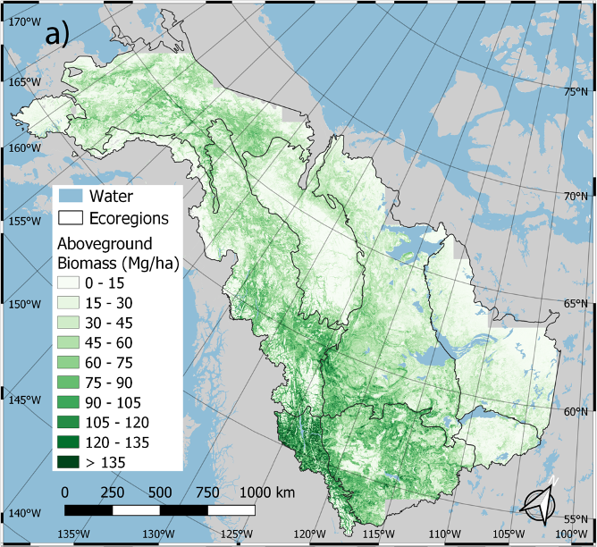
Figure 1. Spatial distribution of predicted aboveground biomass (AGB) density averaged over 1984-2014 for the ABoVE Core Study Domain. Solid black lines indicate the EPA Level 2 Ecoregion boundaries. Source: Wang et al. (2021)
Citation
Wang, J., M.K. Farina, A. Baccini, and M.A. Friedl. 2021. ABoVE: Annual Aboveground Biomass for Boreal Forests of ABoVE Core Domain, 1984-2014. ORNL DAAC, Oak Ridge, Tennessee, USA. https://doi.org/10.3334/ORNLDAAC/1808
Table of Contents
- Dataset Overview
- Data Characteristics
- Application and Derivation
- Quality Assessment
- Data Acquisition, Materials, and Methods
- Data Access
- References
Dataset Overview
This dataset provides estimated annual aboveground biomass (AGB) density for live woody (tree and shrub) species and corresponding standard errors at a 30 m spatial resolution for the boreal forest biome portion of the Core Study Domain of NASA's Arctic-Boreal Vulnerability Experiment (ABoVE) Project (Alaska and Canada) over the time period 1984-2014. The data were derived from a time series of Landsat-5 and Landsat-7 surface reflectance imagery and full-waveform lidar returns from the Geoscience Laser Altimeter System (GLAS) flown onboard IceSAT from 2004 to 2008. The Change Detection and Classification (CCDC) model-fitting algorithm was used to estimate the seasonal variability in surface reflectance, and AGB density data were produced by applying allometric equations to the GLAS lidar data. A Gradient Boosted Machines machine learning algorithm was used to predict annual AGB density across the study domain given the seasonal variability in surface reflectance and other predictors. The data received statistical smoothing to reduce noise and uncertainty was estimated at the pixel level. These data contribute to the characterization of how biomass stocks are responding to climate and disturbance in boreal forests.
Data are provided in the ABoVE standard Albers equal area conic projection (30 m spatial resolution) and are gridded into 180x180 km ABoVE standard “B” grid tiles (Loboda et al., 2019). For this study, there are a total of 106 grid tiles over the ABoVE Core Study Domain.
Project: Arctic-Boreal Vulnerability Experiment
The Arctic-Boreal Vulnerability Experiment (ABoVE) is a NASA Terrestrial Ecology Program field campaign being conducted in Alaska and western Canada, for 8 to 10 years, starting in 2015. Research for ABoVE links field-based, process-level studies with geospatial data products derived from airborne and satellite sensors, providing a foundation for improving the analysis, and modeling capabilities needed to understand and predict ecosystem responses to, and societal implications of, climate change in the Arctic and Boreal regions.
Related Publication
Wang, J.A., A. Baccini, M.K. Farina, J.T. Randerson, and M.A. Friedl. 2021. Disturbance suppresses the aboveground biomass carbon sink in North American boreal forests. In revision at Nature Climate Change.
Related Dataset
Wang, J.A., D. Sulla-Menashe, C.E. Woodcock, O. Sonnentag, R.F. Keeling, and M.A. Friedl. 2019. ABoVE: Landsat-derived Annual Dominant Land Cover Across ABoVE Core Domain, 1984-2014. ORNL DAAC, Oak Ridge, Tennessee, USA. https://doi.org/10.3334/ORNLDAAC/1691
Acknowledgments
This work was supported by NASA ABoVE (grant NNX15AU63A), NASA MeASUREs (grant 80NSSC18K0994), and NSF GRFP (grant DGE-1247312).
Data Characteristics
Spatial Coverage: Boreal forest areas of Alaska and Canada
ABoVE Reference Locations
Domain: Core ABoVE
Data are provided in the ABoVE standard Albers equal area conic projection
State/Territory: Alaska
Grid Cells (106): Bh01v04, Bh01v05, Bh02v03, Bh02v04, Bh02v05, Bh03v03, Bh03v04, Bh03v05, Bh04v03, Bh04v04, Bh04v05, Bh05v03, Bh05v04, Bh05v05, Bh05v06, Bh06v03, Bh06v04, Bh06v05, Bh06v06, Bh06v07, Bh06v08, Bh06v09, Bh07v04, Bh07v05, Bh07v06, Bh07v07, Bh07v08, Bh07v09, Bh07v10, Bh08v04, Bh08v05, Bh08v06, Bh08v07, Bh08v08, Bh08v09, Bh08v10, Bh08v11, Bh08v12, Bh08v13, Bh08v14, Bh09v05, Bh09v06, Bh09v07, Bh09v08, Bh09v09, Bh09v10, Bh09v11, Bh09v12, Bh09v13, Bh09v14, Bh09v15, Bh10v05, Bh10v06, Bh10v07, Bh10v08, Bh10v09, Bh10v10, Bh10v11, Bh10v12, Bh10v13, Bh10v14, Bh10v15, Bh10v16, Bh11v06, Bh11v07, Bh11v08, Bh11v09, Bh11v10, Bh11v11, Bh11v12, Bh11v13, Bh11v14, Bh11v15, Bh11v16, Bh12v08, Bh12v09, Bh12v10, Bh12v11, Bh12v12, Bh12v13, Bh12v14, Bh12v15, Bh13v08, Bh13v09, Bh13v10, Bh13v11, Bh13v12, Bh13v13, Bh13v14, Bh13v15, Bh14v09, Bh14v10, Bh14v11, Bh14v12, Bh14v13, Bh14v14, Bh14v15, Bh15v11, Bh15v12, Bh15v13, Bh15v14, Bh15v15, Bh16v11, Bh16v12, Bh16v13, Bh16v14
Spatial Resolution: 30 m
Temporal Coverage: 1984-01-01 to 2014-12-31 (31 years)
Temporal Resolution: Annual
Study Area: Latitude and longitude are given in decimal degrees.
| Site | Northernmost Latitude | Southernmost Latitude | Easternmost Longitude | Westernmost Longitude |
|---|---|---|---|---|
| Alaska and Canada | 69.7323361 | 51.7769389 | -101.736394 | -165.4101389 |
Data File Information
There are 212 files in geoTIFF (*.tif) format included in this dataset; 106 files of estimated AGB for each tile and 106 files of corresponding standard errors for estimated AGB. Each file has 31 bands, one for each year of data (from 1984 to 2014, inclusive). The first band is the year 1984, the second band is the year 1985, and so on through to the 31st band being the year 2014.
File Naming Convention
This dataset uses the ABoVE standard Albers equal area conic projection (30 m spatial resolution) and is gridded into 180x180 km ABoVE standard “B” grid tiles. There are a total of 106 B grid tiles over the ABoVE core domain in this dataset. Each of the resulting data filenames includes the respective ABoVE Standard B grid tile coordinates (BhHHvVV). The respective ABoVE standard "B" grid tiles can be identified based on location by using the shapefiles provided in the related dataset (Loboda et al., 2019; https://doi.org/10.3334/ORNLDAAC/1527).
The files are named ABoVE_variable_BhHHvVV.tif (e.g., ABoVE_AGB_Bh01v04.tif, ABoVE_AGB_SE_Bh01v04.tif), where
- variable = AGB or AGB_SE
- HH = 01-16, the horizontal ABoVE B grid tile location
- VV = 03-16, the vertical ABoVE B grid tile location
Table 1. File names and descriptions.
| File Names | Units | Description |
|---|---|---|
| ABoVE_AGB_BhHHvVV.tif | Mg ha-1 | Estimated live aboveground woody (tree and shrub) biomass (AGB) in megagrams of carbon per hectare. There is a scale factor of 0.01. |
| ABoVE_AGB_SE_BhHHvVV.tif | Mg ha-1 | The standard error of estimated live AGB in megagrams of carbon per hectare. There is a scale factor of 0.01. |
Data File Details
For each file,
- There are 31 bands that correspond to the time period 1984-2014, where band 1 is the year 1984, band 31 is 2014, etc.
- Missing values are represented by "65535."
- The spatial reference system is "Canada_Albers_Equal_Area_Conic" (EPSG:102001), PROJ4:+proj=aea +lat_1=50 +lat_2=70 +lat_0=40 +lon_0=-96 +x_0=0 +y_0=0 +datum=NAD83 +units=m +no_defs.
- There are 6000 rows and 6000 columns (180 km x 180 km) in a "B" grid tile.
- The data have a scale factor of 0.01. Provided values should be multiplied by the scale factor to obtain true values.
Application and Derivation
Boreal forests are a critical component of the global carbon cycle due to their vast extent, climate sensitivity, and the immense amount of carbon they store in biomass and organic soils. Accurate characterization of how biomass stocks are responding to climate and disturbance is essential to understanding recent and future changes in the northern high-latitude terrestrial carbon sink. Prior to this study, however, remote sensing-based maps of AGB in boreal forests typically cover a single period, precluding analysis of temporal dynamics arising from climate change or disturbance. These data were used to quantify how disturbances influence boreal AGB trends, how this influence is changing over time, and how estimates of AGB stocks and changes compare to estimates from earth system models used to forecast climate change.
Quality Assessment
The accuracy of the AGB model was primarily assessed from a 20% hold-out independent validation dataset used in the Gradient Boosted Machines assessment. The model predicted AGB with R2 = 0.8001 and RMSE = 20.77 Mg ha-1. The estimates of the stocks and uncertainties of AGB were compared to the equivalent domain and similar time periods from four other remote sensing-based AGB datasets, including those developed by the North American Carbon Program (Margolis et al., 2015), the European Space Agency (Santoro and Cartus, 2019), the Canadian Forest Service (Matasci et al., 2018), and Spawn et al. (2020). The model estimates for both the AGB density and the AGB stocks matched fairly well within the range of those comparable datasets.
There tended to be a slight low bias at high values of AGB density; that is the data are slightly underestimated within dense forests. Several instances where CCDC was unable to fit a model, likely because of lack of clear observations, resulted in missing values, primarily at mountain tops and in very cold areas with a limited growing season length.
Data Acquisition, Materials, and Methods
Study Area
The study is focused on the ABoVE Core Study Domain, a vast region of Alaska and western Canada that comprises 4.7 x 10⁶ km2. Excluded areas included regions considered tundra according to the EPA’s Level 2 Ecoregions for North America, and ecoregions with limited overlap with the ABoVE Core Study Domain and limited to observed aboveground live woody biomass (AGB) stocks (e.g., Marine West Coast Forest, Temperate Prairies). The resulting area was 2,821,806 km2. Only AGB in trees and shrubs were considered and not other carbon stocks (e.g., dead wood, coarse woody debris, litter, and soil organic matter).
Data Processing
The data processing workflow consisted of five main parts: (1) preprocessing of Landsat surface reflectance data, (2) estimation of Landsat seasonal-spectral data using the Change Detection and Classification (CCDC) model-fitting algorithm; (3) production of AGB density data by applying allometric equations to spaceborne lidar data from the Geoscience Laser Altimeter System (GLAS); (4) fitting and applying the Gradient Boosted Machines machine learning algorithm to predict annual AGB density across the study domain; and (5) a statistical smoothing technique to reduce noise and estimate uncertainty at the pixel level (Figure 2).
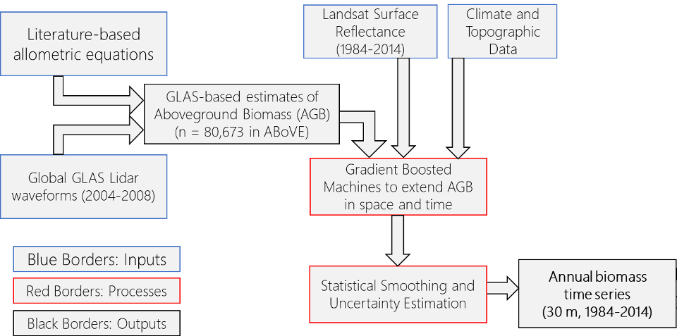
Figure 2. Flowchart detailing the inputs, computational processes, and outputs involved in the creation of this dataset. Source: Wang et al. (2021)
1. Preprocessing of Landsat Surface Reflectance Data
A time series of 30 m surface reflectance data from the Thematic Mapper (TM) onboard Landsat-5 and the Enhanced Thematic Mapper Plus (ETM+) onboard Landsat-7 were collected for the time period 1984–2014. The Landsat surface reflectance data were masked for ephemeral contamination using the Fmask algorithm (Zhu and Woodcock, 2012). The area mapped was defined by an ocean-land mask that was adopted from a 10 m ocean mask from the Natural Earth data repository (Kelso and Patterson, 2010) and manually edited to closely fit the coastline of the study region. Data within the “tundra” areas (i.e., EPA NA CODE=2) of the EPA Level 1 North America ecoregions (Omernik and Griffith, 2014) were removed.
2. CCDC Model Fitting
Reflectance data from each Landsat standard WRS2 row/path scene was reprojected into the ABoVE defined Albers equal area conic projection, 30 m spatial resolution, and tiled into the ABoVE reference grid; a standard used by all ABoVE projects (Loboda et al. 2019). The CCDC algorithm (Zhu and Woodcock, 2014) was used to detect statistical breaks in the time series of the Landsat surface reflectance data and to model seasonal variability in surface reflectance. For each year at each pixel, the CCDC algorithm was used to fit piecewise harmonic models to the Landsat surface reflectance data at each 30 m pixel. Then the mean growing season and non-growing season values for each of the six spectral reflectance bands (e.g., normalized difference vegetation index) were calculated, resulting in estimated Landsat seasonal-spectral data. Because the CCDC models can be unstable when growing seasons are short (i.e., fewer than 100 days), the snow-free growing season was normalized to the 5th and 95th percentiles of the snow-free days of the year at each pixel. Areas classified as “herbaceous” throughout the entire period were not included in the analysis.
3. GLAS-Based Estimation of AGB
Allometric equations retrieved from existing literature (see Wang et al., 2020) were applied to forest height metrics derived from full-waveform lidar data from GLAS/ICESat L1A Global Altimetry Data (HDF5), Version 33 (Zwally et al. 2013), that flew onboard ICESat from 2003 through 2009. Data from the Canadian Earth Observation for Sustainable Development land cover dataset (Wulder et al., 2008), the Alaskan National Land Cover Database (Jin et al., 2017), the Ecoregions2017 ecoregion numbers (Dinerstein et al., 2017), and the MODIS global burned area product (MCD45; Roy et al., 2008) were used in the allometric equations to derive AGB density for each GLAS observation. For quality control, ASTER digital elevation models (Tachikawa et al. 2011) were used to exclude data on terrain that had slopes greater than 10 degrees, and annual land cover maps for the ABoVE Domain (Wang et al., 2019) were used to exclude data that fell within areas of heterogeneous land cover. This yielded 80,673 GLAS-based estimates of AGB.
4. Application of Gradient Boosted Machines Algorithm
The GLAS-derived estimates of AGB were used as a response variable and the estimated Landsat seasonal-spectral data were used as predictor variables in an ensemble machine learning model called Gradient Boosted Machines (Greenwell et al., 2019). Long-term mean annual temperature and precipitation from WorldClim (Fick and Hijmans, 2017) and annual land cover (Wang et al. 2019) were also used as predictors. The mlr package in R (Bischl et al. 2016) was used to tune hyperparameters for the model. The resulting model was applied across the ABoVE Core Study Domain.
5. Statistical Smoothing
The initial time series of GLAS-based AGB at each pixel showed non-negligible interannual variation, resulting in many instances of spurious changes in AGB. Following the methodology of Baccini et al. (2017), this issue was resolved using a temporal change-point algorithm that fits piecewise linear models to the pixel-wise time series of AGB. Pixel-level changes in AGB were evaluated on the basis of the temporal segmentation and linear model fits, rather than the Gradient Boosted Machine-predicted biomass values themselves.
Data Access
These data are available through the Oak Ridge National Laboratory (ORNL) Distributed Active Archive Center (DAAC).
ABoVE: Annual Aboveground Biomass for Boreal Forests of ABoVE Core Domain, 1984-2014
Contact for Data Center Access Information:
- E-mail: uso@daac.ornl.gov
- Telephone: +1 (865) 241-3952
References
Baccini, A., W. Walker, L. Carvalho, M. Farina, D. Sulla-Menashe, and R.A. Houghton. 2017. Tropical forests are a net carbon source based on aboveground measurements of gain and loss. Science 358:230–234. https://doi.org/10.1126/science.aam5962
Bischl, B., M. Lang, L. Kotthoff, J. Schiffner, J. Richter, E. Studerus, G. Casalicchio, and Z.M. Jones. 2016. Mlr: machine learning in R. The Journal of Machine Learning Research 17(1):5938–5942. http://jmlr.org/papers/v17/15-066.html
Dinerstein, E., D. Olson, A. Joshi, C. Vynne, N.D. Burgess, E. Wikramanayake, et al. 2017. An Ecoregion-Based Approach to Protecting Half the Terrestrial Realm. BioScience 67:534–545.https://doi.org/10.1093/biosci/bix014
Fick, S. E., and R. J. Hijmans. 2017. WorldClim 2: new 1-km spatial resolution climate surfaces for global land areas. International Journal of Climatology 37:4302–4315. https://doi.org/10.1002/joc.5086
Greenwell, B., Boehmke, B., Cunningham, J., and GBM Developers. 2019. gbm: Generalized Boosted Regression Models. R package version 2.1.8.
Jin, S., L. Yang, Z. Zhu, and C. Homer. 2017. A land cover change detection and classification protocol for updating Alaska NLCD 2001 to 2011. Remote Sensing of Environment 195:44–55. https://doi.org/10.1016/j.rse.2017.04.021
Kelso, N.V., and T. Patterson. 2010. Introducing natural earth data - naturalearthdata.com. Geographia Technica 5, 82–89.
Loboda, T.V., E.E. Hoy, and M.L. Carroll. 2019. ABoVE: Study Domain and Standard Reference Grids, Version 2. ORNL DAAC, Oak Ridge, Tennessee, USA. https://doi.org/10.3334/ORNLDAAC/1527
Margolis, H., G. Sun, P.M. Montesano, and R.F. Nelson. 2015. NACP LiDAR-based Biomass Estimates, Boreal Forest Biome, North America, 2005-2006. ORNL DAAC, Oak Ridge, Tennessee, USA. https://doi.org/10.3334/ORNLDAAC/1273
Matasci, G., T. Hermosilla, M.A. Wulder, J.C. White, N.C. Coops, G.W. Hobart, D.K. Bolton, P. Tompalski, and C.W. Bater. 2018. Three decades of forest structural dynamics over Canada’s forested ecosystems using Landsat time-series and lidar plots. Remote Sensing of Environment 216:697–714. https://doi.org/10.1016/j.rse.2018.07.024
Omernik, J.M., and G.E. Griffith. 2014. Ecoregions of the conterminous United States: evolution of a hierarchical spatial framework. Environmental Management 54, 1249–1266. https://doi.org/10.1007/s00267-014-0364-1
Roy, D.P., L. Boschetti, C.O. Justice, and J. Ju. 2008. The collection 5 MODIS burned area product — Global evaluation by comparison with the MODIS active fire product. Remote Sensing of Environment 112:3690–3707.https://doi.org/10.1016/j.rse.2008.05.013
Santoro, M., and O. Cartus. 2019. ESA Biomass Climate Change Initiative (Biomass_cci): Global datasets of forest above-ground biomass for the year 2017, v1. Centre for Environmental Data Analysis (CEDA). https://doi.org/10.5285/bedc59f37c9545c981a839eb552e4084
Spawn, S.A., and H.K. Gibbs. 2020. Global Aboveground and Belowground Biomass Carbon Density Maps for the Year 2010. ORNL DAAC, Oak Ridge, Tennessee, USA. https://doi.org/10.3334/ORNLDAAC/1763
Tachikawa, T., M. Hato, M. Kaku, and A. Iwasaki. 2011. Characteristics of ASTER GDEM version 2. Page 2011 IEEE International Geoscience and Remote Sensing Symposium. IEEE. https://doi.org/10.1109/IGARSS.2011.6050017
Wang, J.A., D. Sulla-Menashe, C.E. Woodcock, O. Sonnentag, R.F. Keeling, and M.A. Friedl. 2019. ABoVE: Landsat-derived Annual Dominant Land Cover Across ABoVE Core Domain, 1984-2014. ORNL DAAC, Oak Ridge, Tennessee, USA. https://doi.org/10.3334/ORNLDAAC/1691
Wulder, MA., J.C. White, M. Cranny, R.J. Hall, J.E. Luther, A. Beaudoin, D.G. Goodenough, and J.A. Dechka. 2008. Monitoring Canada’s forests. Part 1: Completion of the EOSD land cover project. Canadian Journal of Remote Sensing 34(6):549–562. https://doi.org/10.5589/m08-066
Zhu, Z., and C.E. Woodcock. 2012. Object-based cloud and cloud shadow detection in Landsat imagery. Remote Sensing of Environment 118:83–94. https://doi.org/10.1016/j.rse.2011.10.028
Zhu, Z., and C.E. Woodcock. 2014. Continuous change detection and classification of land cover using all available Landsat data. Remote Sensing of Environment 144:152–171. https://doi.org/10.1016/j.rse.2014.01.011
Zwally, H.J., R. Schutz, C. Bentley, J. Bufton, T. Herring, J. Minster, J. Spinhirne, and R. Thomas. 2013. GLAS/ICESat L1A Global Altimetry Data (HDF5), Version 33. Boulder, Colorado USA. NASA National Snow and Ice Data Center Distributed Active Archive Center. https://doi.org/10.5067/ICESAT/GLAS/DATA101