Documentation Revision Date: 2021-08-27
Dataset Version: 1
Summary
Continuous-cover field maps have many advantages over traditional thematic maps, and the methods used here are well-suited to support periodic cover updates in tandem with future field and Landsat observations.
There are 39 data files included in this dataset. Continuous coverage data are provided in GeoTIFF (*.tif) format for 19 field cover types, each in two projections: Alaska Albers Equal Area Conic (EPSG:3338) and the ABoVE standard projection, Canada Albers Equal Area Conic (EPSG:102001) for a total of 38 files. The field data and predictors used in modeling are provided in one comma-separated file (*.csv).
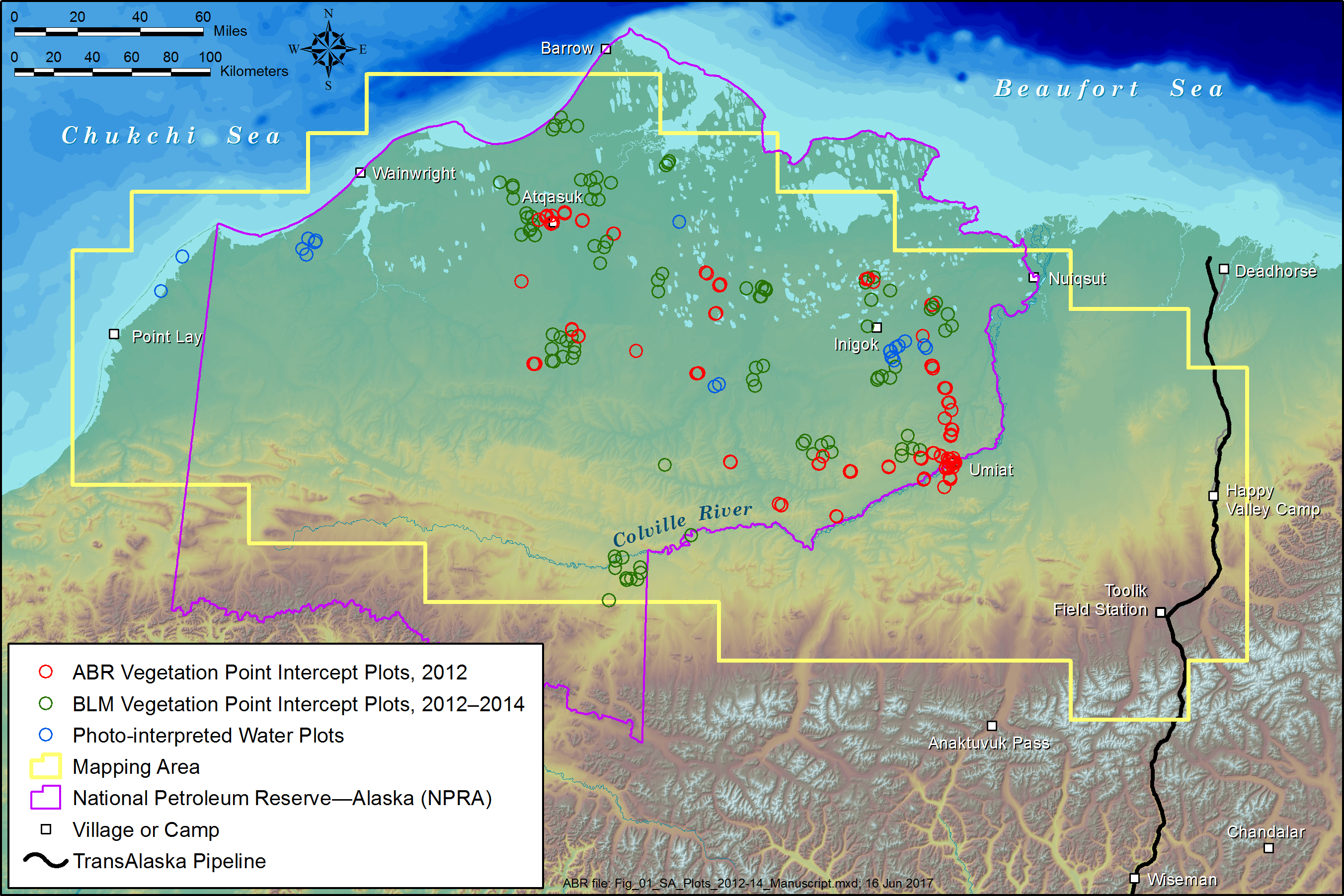
Figure 1. Map of quantitative-cover mapping area showing the distribution of field plots, North Slope, Alaska. ABR is ABR, Inc.-Environmental Research & Services and BLM is the Bureau of Land Management. Source: Macander et al., 2017
Citation
Macander, M.J., G.V. Frost, P.R. Nelson, and C.S. Swingley. 2020. ABoVE: Tundra Plant Functional Type Continuous-Cover, North Slope, Alaska, 2010-2015. ORNL DAAC, Oak Ridge, Tennessee, USA. https://doi.org/10.3334/ORNLDAAC/1830
Table of Contents
- Dataset Overview
- Data Characteristics
- Application and Derivation
- Quality Assessment
- Data Acquisition, Materials, and Methods
- Data Access
- References
Dataset Overview
This dataset provides predicted continuous-field cover for tundra plant functional types (PFTs), across ~125,000 km2 of Alaska's North Slope at 30 m resolution. The data cover the period 2010-07-01 to 2015-08-31. The data were derived using a random forest data-mining algorithm, predictors derived from Landsat satellite observations (surface reflectance composites for ~15-day periods from May-August), and field vegetation cover and site characterization data spanning bioclimatic and geomorphic gradients. The field vegetation cover was stratified by nine PFTs, plus open water, bare ground, and litter, and using the cover metrics total cover (areal cover including the understory) and top cover (uppermost canopy or ground cover), resulting in a total of 19 field cover types. The field data and predictor values at the field sites are also included.
Continuous-cover field maps have many advantages over traditional thematic maps, and the methods used here are well-suited to support periodic cover updates in tandem with future field and Landsat observations.
Project: Arctic-Boreal Vulnerability Experiment
The Arctic-Boreal Vulnerability Experiment (ABoVE) is a NASA Terrestrial Ecology Program field campaign based in Alaska and western Canada between 2016 and 2021. Research for ABoVE links field-based, process-level studies with geospatial data products derived from airborne and satellite sensors, providing a foundation for improving the analysis and modeling capabilities needed to understand and predict ecosystem responses and societal implications.
Related Publication
Macander, M., G. Frost, P. Nelson, and C. Swingley. 2017. Regional Quantitative Cover Mapping of Tundra Plant Functional Types in Arctic Alaska. Remote Sensing 9:1024. https://doi.org/10.3390/rs9101024
Related Datasets
For datasets related to vegetation in Alaska refer to additional ABoVE datasets.
Acknowledgments
This study was funded by the NASA ABoVE project (grant NNX17AE44G).
Data Characteristics
Spatial Coverage: Alaska’s North Slope
ABoVE Reference Locations
Domain: Core ABoVE
Grid cells (30 m): Bh006v000, Bh007v000, Bh006v001, Bh007v001, Bh008v001, Bh006v002, Bh007v002, Bh008v002, Bh007v003, Bh008v003
Spatial Resolution: 30 m
Temporal Coverage: 2010-05-16 to 2015-08-31
Temporal Resolution: One-time estimates
Study Area: Latitude and longitude are given in decimal degrees.
| Sites | Westernmost Longitude | Easternmost Longitude | Northernmost Latitude | Southernmost Latitude |
|---|---|---|---|---|
| North Slope | -167.4761 | -143.978 | 73.8004 | 65.5858 |
Data file information
There are 39 data files included in this dataset. Continuous coverage data are provided in GeoTIFF (*.tif) format for 19 field cover types, each in two projections: Alaska Albers Equal Area Conic (EPSG:3338) and the ABoVE standard projection, Canada Albers Equal Area Conic (EPSG:102001) for a total of 38 files. The field data and predictors used in modeling are provided in one comma-separated file (*.csv) Model_Training_Testing_Data.csv. The 133 variables are described in Table 2.
The GeoTIFF files are named according to the PFT and summarized measurements of the PFTs (Table 3) and cover metrics total cover (areal cover including the understory) and top cover (uppermost canopy or ground cover). The data are continuous-field percent ground cover for PFTs at 30 m resolution across ~125,000 km² of Alaska’s North Slope.
Table 1. GeoTIFF File Names. The PFTs and other cover types are described in Table 3.
| Files in Alaska Albers Equal Area Conic Projection (EPSG:3338) | Files in ABoVE Standard Projection (EPSG:102001) |
|---|---|
| Bare_Ground_Top_Cover.tif | Bare_Ground_Top_Cover_102001.tif |
| Bryophyte_Total_Cover.tif | Bryophyte_Total_Cover_102001.tif |
| Dwarf_Deciduous_Shrub_Total_Cover.tif | Dwarf_Deciduous_Shrub_Total_Cover_102001.tif |
| Dwarf_Evergreen_Shrub_Total_Cover.tif | Dwarf_Evergreen_Shrub_Total_Cover_102001.tif |
| Forb_Total_Cover.tif | Forb_Total_Cover_102001.tif |
| Grass_Total_Cover.tif | Grass_Total_Cover_102001.tif |
| Lichen_Total_Cover.tif | Lichen_Total_Cover_102001.tif |
| Litter_Top_Cover.tif | Litter_Top_Cover_102001.tif |
| Low_and_Tall_Deciduous_Shrub_Total_Cover.tif | Low_and_Tall_Deciduous_Shrub_Total_Cover_102001.tif |
| Low_Deciduous_Shrub_Total_Cover.tif | Low_Deciduous_Shrub_Total_Cover_102001.tif |
| Nonvascular_Plant_Top_Cover.tif | Nonvascular_Plant_Top_Cover_102001.tif |
| Nonvascular_Plant_Total_Cover.tif | Nonvascular_Plant_Total_Cover_102001.tif |
| Open_Water_Top_Cover.tif | Open_Water_Top_Cover_102001.tif |
| Sedge_Total_Cover.tif | Sedge_Total_Cover_102001.tif |
| Tall_Deciduous_Shrub_Total_Cover.tif | Tall_Deciduous_Shrub_Total_Cover_102001.tif |
| Total_Herbaceous_Total_Cover.tif | Total_Herbaceous_Total_Cover_102001.tif |
| Total_Shrub_Total_Cover.tif | Total_Shrub_Total_Cover_102001.tif |
| Vascular_Plant_Top_Cover.tif | Vascular_Plant_Top_Cover_102001.tif |
| Vascular_Plant_Total_Cover.tif | Vascular_Plant_Total_Cover_102001.tif |
Data File Details
For all geoTIFF files:
- There are two projections; Alaska Albers Equal Area Conic (EPSG:3338) and the ABoVE standard projection, Canada Albers Equal Area Conic (EPSG:102001)
- The no data value is represented by "255"
- There is a single bands
- Map units are in meters
Table 2. Variables in the file Model_Training_Testing Data.csv. User Note: Many of the variables have a scale factor. All spectral indices are "Scaled by factor of 10000". Slope and snow free days have a scale factor of 100. Elevation is reported in decimeters.
| Variable | Units | Description |
|---|---|---|
| plot_id | Unique name identifying the sample location | |
| sample_date | YYYY-MM-DD | Date when field sampling occurred |
| line_length | m | Length of each sampling line |
| plot_radius | m | Radius of plot |
| source | Name of the field sampling campaign (ABR 2012, NPRA AIM, ABR Office) described in Section 5. | |
| longitude | decimal degrees | Longitude in decimal degrees |
| latitude | decimal degrees | Latitude in decimal degrees |
| x_coord | m | X coordinate, EPSG 3338 |
| y_coord | m | Y coordinate, EPSG 3338 |
| train_test | Identifies whether data was in the training or reserved validation set | |
| totalcover_shrubs | % | Total cover of shrubs |
| totalcover_d_low_tall_shrubs | % | Total cover of deciduous low and tall shrubs |
| totalcover_d_tall_shrubs | % | Total cover of deciduous tall shrubs |
| totalcover_d_low_shrubs | % | Total cover of deciduous low shrubs |
| totalcover_d_shrubs | % | Total cover of deciduous shrubs |
| totalcover_e_shrubs | % | Total cover of evergreen shrubs |
| totalcover_sedges_rush | % | Total cover of sedges and rushes |
| totalcover_grasses | % | Total cover of grasses |
| totalcover_forbs_ferns | % | Total cover of forbs and ferns |
| totalcover_vascular | % | Total cover of vascular plants |
| totalcover_nonvascular | % | Total cover of nonvascular plants |
| totalcover_mosses | % | Total cover of mosses |
| totalcover_lichens | % | Total cover of lichens |
| totalcover_liverworts | % | Total cover of liverworts |
| totalcover_algae | % | Total cover of algae |
| totalcover_dwarfshrub | % | Total cover of dwarf shrub |
| totalcover_herbs | % | Total cover of herbs (grasses, sedges, forbs) |
| totalcover_bryophytes | % | Total cover of bryophytes (liverworts and mosses) |
| topcover_shrubs | % | Top cover of shrubs |
| topcover_d_low_tall_shrubs | % | Top cover of deciduous low and tall shrubs |
| topcover_d_tall_shrubs | % | Top cover of deciduous tall shrubs |
| topcover_d_low_shrubs | % | Top cover of deciduous low shrubs |
| topcover_d_shrubs | % | Top cover of deciduous shrubs |
| topcover_e_shrubs | % | Top cover of evergreen shrubs |
| topcover_sedges_rush | % | Top cover of sedges and rushes |
| topcover_grasses | % | Top cover of grasses |
| topcover_forbs_ferns | % | Top cover of forbs and ferns |
| topcover_vascular | % | Top cover of vascular plants |
| topcover_nonvascular | % | Top cover of nonvascular plants |
| topcover_mosses | % | Top cover of mosses |
| topcover_lichens | % | Top cover of lichens |
| topcover_liverworts | % | Top cover of liverworts |
| topcover_algae | % | Top cover of algae |
| topcover_litter | % | Top cover of litter |
| topcover_water | % | Top cover of water |
| topcover_bareground | % | Top cover of bare ground |
| mean_woody_height | cm | Mean woody height by AIM method |
| woody_se | cm | Standard error of woody height by AIM method |
| count_woody_height | Count of height points where woody vegetation was present | |
| mean_herb_height | cm | Mean herbaceous height by AIM method |
| herb_se | cm | Standard error of herbaceous height by AIM method |
| count_herb_height | Count of height points where herbaceous vegetation was present | |
| count_heights_sampled | Count of height points | |
| count_points_sampled | Count of vegetation point intercept points | |
| vascular_species_richness | Vascular species richness | |
| band1i_l_spr | Scaled by factor of 10000 | Spring surface reflectance, Landsat 7 band 1 |
| band2i_l_spr | Scaled by factor of 10000 | Spring surface reflectance, Landsat 7 band 2 |
| band3i_l_spr | Scaled by factor of 10000 | Spring surface reflectance, Landsat 7 band 3 |
| band4i_l_spr | Scaled by factor of 10000 | Spring surface reflectance, Landsat 7 band 4 |
| band5i_l_spr | Scaled by factor of 10000 | Spring surface reflectance, Landsat 7 band 5 |
| band7i_l_spr | Scaled by factor of 10000 | Spring surface reflectance, Landsat 7 band 6 |
| ndvi_l_spr | Scaled by factor of 10000 | Spring Normalized Difference Vegetation Index (NDVI) |
| nbr_l_spr | Scaled by factor of 10000 | Spring Normalized Burn Ratio (NBR) |
| ndmi_l_spr | Scaled by factor of 10000 | Spring Normalized Difference Moisture Index (NDMI) |
| ndsi_l_spr | Scaled by factor of 10000 | Spring Normalized Difference Snow Index (NDSI) |
| ndwi_l_spr | Scaled by factor of 10000 | Spring Normalized Difference Water Index (NDWI) |
| evi2_l_spr | Scaled by factor of 10000 | Spring Enhanced Vegetation Index (EVI) |
| band1i_l_0608 | Scaled by factor of 10000 | Early June surface reflectance, Landsat 7 band 1 |
| band2i_l_0608 | Scaled by factor of 10000 | Early June surface reflectance, Landsat 7 band 2 |
| band3i_l_0608 | Scaled by factor of 10000 | Early June surface reflectance, Landsat 7 band 3 |
| band4i_l_0608 | Scaled by factor of 10000 | Early June surface reflectance, Landsat 7 band 4 |
| band5i_l_0608 | Scaled by factor of 10000 | Early June surface reflectance, Landsat 7 band 5 |
| band7i_l_0608 | Scaled by factor of 10000 | Early June surface reflectance, Landsat 7 band 6 |
| ndvi_l_0608 | Scaled by factor of 10000 | Early June NDVI |
| nbr_l_0608 | Scaled by factor of 10000 | Early June NBR |
| ndmi_l_0608 | Scaled by factor of 10000 | Early June NDMI |
| ndsi_l_0608 | Scaled by factor of 10000 | Early June NDSI |
| ndwi_l_0608 | Scaled by factor of 10000 | Early June NDWI |
| evi2_l_0608 | Scaled by factor of 10000 | Early June EVI |
| band1i_l_0623 | Scaled by factor of 10000 | Late June surface reflectance, Landsat 7 band 1 |
| band2i_l_0623 | Scaled by factor of 10000 | Late June surface reflectance, Landsat 7 band 2 |
| band3i_l_0623 | Scaled by factor of 10000 | Late June surface reflectance, Landsat 7 band 3 |
| band4i_l_0623 | Scaled by factor of 10000 | Late June surface reflectance, Landsat 7 band 4 |
| band5i_l_0623 | Scaled by factor of 10000 | Late June surface reflectance, Landsat 7 band 5 |
| band7i_l_0623 | Scaled by factor of 10000 | Late June surface reflectance, Landsat 7 band 6 |
| ndvi_l_0623 | Scaled by factor of 10000 | Late June NDVI |
| nbr_l_0623 | Scaled by factor of 10000 | Late June NBR |
| ndmi_l_0623 | Scaled by factor of 10000 | Late June NDMI |
| ndsi_l_0623 | Scaled by factor of 10000 | Late June NDSI |
| ndwi_l_0623 | Scaled by factor of 10000 | Late June NDWI |
| evi2_l_0623 | Scaled by factor of 10000 | Late June EVI |
| band1i_l_0708 | Scaled by factor of 10000 | Early July surface reflectance, Landsat 7 band 1 |
| band2i_l_0708 | Scaled by factor of 10000 | Early July surface reflectance, Landsat 7 band 2 |
| band3i_l_0708 | Scaled by factor of 10000 | Early July surface reflectance, Landsat 7 band 3 |
| band4i_l_0708 | Scaled by factor of 10000 | Early July surface reflectance, Landsat 7 band 4 |
| band5i_l_0708 | Scaled by factor of 10000 | Early July surface reflectance, Landsat 7 band 5 |
| band7i_l_0708 | Scaled by factor of 10000 | Early July surface reflectance, Landsat 7 band 6 |
| ndvi_l_0708 | Scaled by factor of 10000 | Early July NDVI |
| nbr_l_0708 | Scaled by factor of 10000 | Early July NBR |
| ndmi_l_0708 | Scaled by factor of 10000 | Early July NDMI |
| ndsi_l_0708 | Scaled by factor of 10000 | Early July NDSI |
| ndwi_l_0708 | Scaled by factor of 10000 | Early July NDWI |
| evi2_l_0708 | Scaled by factor of 10000 | Early July EVI |
| band1i_l_0801 | Scaled by factor of 10000 | Midsummer surface reflectance, Landsat 7 band 1 |
| band2i_l_0801 | Scaled by factor of 10000 | Midsummer surface reflectance, Landsat 7 band 2 |
| band3i_l_0801 | Scaled by factor of 10000 | Midsummer surface reflectance, Landsat 7 band 3 |
| band4i_l_0801 | Scaled by factor of 10000 | Midsummer surface reflectance, Landsat 7 band 4 |
| band5i_l_0801 | Scaled by factor of 10000 | Midsummer surface reflectance, Landsat 7 band 5 |
| band7i_l_0801 | Scaled by factor of 10000 | Midsummer surface reflectance, Landsat 7 band 6 |
| ndvi_l_0801 | Scaled by factor of 10000 | Midsummer NDVI |
| nbr_l_0801 | Scaled by factor of 10000 | Midsummer NBR |
| ndmi_l_0801 | Scaled by factor of 10000 | Midsummer NDMI |
| ndsi_l_0801 | Scaled by factor of 10000 | Midsummer NDSI |
| ndwi_l_0801 | Scaled by factor of 10000 | Midsummer NDWI |
| evi2_l_0801 | Scaled by factor of 10000 | Midsummer EVI |
| band1i_l_0823 | Scaled by factor of 10000 | Late August surface reflectance, Landsat 7 band 1 |
| band2i_l_0823 | Scaled by factor of 10000 | Late August surface reflectance, Landsat 7 band 2 |
| band3i_l_0823 | Scaled by factor of 10000 | Late August surface reflectance, Landsat 7 band 3 |
| band4i_l_0823 | Scaled by factor of 10000 | Late August surface reflectance, Landsat 7 band 4 |
| band5i_l_0823 | Scaled by factor of 10000 | Late August surface reflectance, Landsat 7 band 5 |
| band7i_l_0823 | Scaled by factor of 10000 | Late August surface reflectance, Landsat 7 band 6 |
| ndvi_l_0823 | Scaled by factor of 10000 | Late August NDVI |
| nbr_l_0823 | Scaled by factor of 10000 | Late August NBR |
| ndmi_l_0823 | Scaled by factor of 10000 | Late August NDMI |
| ndsi_l_0823 | Scaled by factor of 10000 | Late August NDSI |
| ndwi_l_0823 | Scaled by factor of 10000 | Late August NDWI |
| evi2_l_0823 | Scaled by factor of 10000 | Late August EVI |
| slope_deg100 | Degrees, scaled by factor of 100 | Terrain slope |
| elevation | Decimeters | Elevation |
| summer_warmth_index100 | Summer warmth index | |
| snowfree_doy100 | Day of year, scaled by factor of 100 | Normal snow-free date |
| p_seas_water100 | % | Water occurrence |
| ndvi_inc | Scaled by factor of 10000 | NDVI amplitude (Midsummer NDVI minus Spring NDVI) |
Application and Derivation
Ecosystem maps are foundational tools that support multi-disciplinary study design and applications including wildlife habitat assessment, monitoring, and earth-system modeling. Continuous-field maps have many advantages over traditional thematic maps. These methods are well-suited to support periodic map updates in tandem with future field and Landsat observations.
Quality Assessment
An assessment of model performance, including root mean squared error, mean absolute error and correlation for each cover type is provided in Macander et al. (2017; Table 4). This assessment was based on both internal cross-validation and iteratively reserving 20% of training data for validation. Selected shrub cover maps were compared to an existing fractional shrub cover map for the North Slope.
Data Acquisition, Materials, and Methods
Study area
The 125,000 km2 mapping area extends from the Chukchi Sea near Point Lay eastward to the Dalton Highway (Fig. 1). The northern half of the mapping area is part of the Arctic Coastal Plain physiographic province (Gallant et al., 1995) characterized by flat topography, poorly drained soils, abundant water bodies, and widespread periglacial landforms such as ice-wedge polygons. Most of the Arctic Coastal Plain corresponds to Bioclimate Subzone D of the Circumpolar Arctic Vegetation Map (CAVM Team, 2003) shrubs are common, but they seldom exceed 1 m in height. The southern half of the mapping area encompasses the Arctic Foothills physiographic province and is characterized by widespread uplands dissected by well-defined drainage networks. The Arctic Foothills is situated in Bioclimate Subzone E, the warmest tundra subzone; shrubs are widespread, and tall thickets (>1.5 m height) are common on floodplains and adjacent slopes, particularly along the Colville River. Hereafter, the two major physiographic provinces are referred to as “coastal plain” and “foothills.” The entire mapping area lies in the zone of continuous permafrost.
Field Data
A field dataset of 106 plots in and near the National Petroleum Reserve-Alaska (NPRA) sampled during July–August 2012 (ABR, 2012) was pooled with 119 plots sampled by the BLM in 2012–2014 as part of the Bureau of Land Management's (BLM) Assessment, Inventory and Monitoring program (NPRA AIM). All field efforts utilized a point-intercept sampling method tailored for long-term monitoring of vegetation (Toevs et al., 2011); this protocol also facilitated sampling at scales appropriate for the analysis of 30 m resolution Landsat data. Plots sampled consisted of three 50 m lines; each line began 5 m from the plot center to avoid vegetation that was trampled during plot setup. The azimuth of the first line was selected randomly, and the others were offset from the first by 120 degrees. Vegetation “hits” were recorded at 1 m intervals using a rod-mounted laser pointer (51 sampling points per line), except at a few plots where logistical constraints necessitated quicker sampling at 2.5 m spacing (21 points per line). At each point, vegetation hits were identified by species by sequentially moving upper canopy leaves aside to allow the laser to hit underlying layers and finally the ground surface. For the ground surface, a single hit was recorded consisting either of live prostrate vegetation, litter, water, or bare ground. Although multiple hits were recorded in the field, only the first live hit for each species was retained for this analysis. The BLM data were collected using the same protocol except that lines were 25 m long and point spacing was 0.5 m (51 points per line).
BLM allocated plots according to a stratified random sampling design based on the 2013 North Slope Science Initiative (NSSI) Land Cover map (NSSI, 2013). Plot locations were subjectively selected in representative vegetation types based on photo signatures evident in 2.5 m resolution aerial imagery. Twenty water-only plots were identified from photo-interpreted satellite imagery within representative areas of clear and turbid water. Water-only plots comprised 9% of the total plot count, which matches the relative extent of open water portrayed on the NSSI map.
For analysis, the cover data were summarized by species, then aggregated to PFTs using two cover metrics: (1) total cover, the percent of sample points at which species belonging to a PFT occurred, summed for all species in a PFT; and (2) top cover, the percent of sample points at which a PFT was the first hit. Total cover values could exceed 100%, but top cover values could not exceed 100%. Importantly, because each species “hit” at a point was recorded and multiple species (including different species of the same PFT) could co-occur at different levels in the canopy, the sum of “total cover” values for all PFTs generally exceeded 100% and occasionally exceeded 100% for a single PFT; for example, in a very dense alder-willow shrubland with >50% cover of both species.
Table 3. Tundra PFTs and other cover types used for cover modeling, North Slope, Alaska (Macander et al., 2017).
| PFT or Other Cover Type | Description | Cover Metric(s) Modeled |
|---|---|---|
| Tall Deciduous Shrubs | Deciduous shrubs ≥1.5 m height; mainly Salix alaxensis, S. arbusculoides and Alnus fruticosa | Total cover |
| Low Deciduous Shrubs | Deciduous shrubs 0.2–1.5 m height; e.g., Betula nana, Salix pulchra, and S. glauca | Total cover |
| Dwarf Deciduous Shrubs | Deciduous shrubs ≤0.2m height; e.g., Salix rotundifolia, Arctous spp., and Vaccinium uliginosum | Total cover |
| Dwarf Evergreen Shrubs | Evergreen shrubs ≤0.2m height; e.g., Dryas integrifolia, Cassiope tetragona, Vaccinium vitis-ideas, and Ledum decumbens | Total cover |
| Sedges | Herbaceous plants of Cyperaceae and Juncaceae; e.g., Carex and Eriophorum spp. | Total cover |
| Grasses | Herbaceous plants of Poaceae; e.g., Arctagrostis, Arctophila, Deschampsia | Total cover |
| Forbs | Non-graminoid herbaceous plants; e.g., legumes and composites | Total cover |
| Mosses | Total of all mosses and liverworts | Total cover |
| Lichens | Total of all ground lichens | Total cover |
| Total Herbaceous | Total of sedges, grasses, and forbs | Total cover |
| Total Shrubs | Total of all shrub PFTs | Total cover |
| Low and Tall Deciduous Shrubs | Deciduous shrubs ≥0.2 m in height | Total cover |
| Vascular Plants | Total of all vascular PFTs | Total and top cover |
| Nonvascular Plants | Total of all nonvascular PFTs including mosses, terricolous | Total and top cover |
| Litter | Dead plant matter | Top cover |
| Open Water | Open water | Top cover |
| Bare Ground | Bare soil or rock | Top cover |
Spectral Predictors: Landsat Seasonal Composites
Calibrated, atmospherically corrected and precision terrain corrected (L1T) Landsat Surface Reflectance High-Level Data Products (Masek et al., 2007) derived from Landsat 4-5 Thematic Mapper (TM), Landsat 7 Enhanced Thematic Mapper (ETM+) and Landsat 8 Operational Land Imager (OLI) observations between 15 May and 31 August 1999–2015 were compiled. This date range captures the spring, summer, and early fall seasons on the North Slope.
Six seasonal Landsat composites were developed to represent ground conditions for key phenological windows from snowmelt to fall senescence using all available Landsat data for a specific date and year ranges. Each composite included six reflective bands as predictors (Table 4).
Table 4. Summary of spectral indices used for cover modeling, North Slope, Alaska.
| Index | Formula | Reference |
|---|---|---|
| Normalized Difference Vegetation Index (NDVI) | (NIR − Red)/(NIR + Red) | Rouse et al., 1974; Tucker et al., 1979 |
| Enhanced Vegetation Index-2 (EVI2) | (Red − Green)/(Red + [2.4 × Green] + 1) | Jiang et al., 2008 |
| Normalized Difference Water Index (NDWI) | (Green − NIR)/(Green + NIR) | McFeeters et al., 1996 |
| Normalized Difference Moisture Index (NDMI) | (NIR − SWIR1)/(NIR + SWIR1) | Goodwin et al., 2008 |
| Normalized Difference Snow Index (NDSI) | (Green − SWIR1)/(Green + SWIR1) | Hall et al., 1995 |
| Normalized Burn Ratio (NBR) | (NIR − SWIR2)/(NIR + SWIR2) | Key et al., 1999 |
To include more potential observations, a one-month seasonal window (16 July–15 August) was used to represent “midsummer”, the period of peak vegetation productivity. A longer year range (1999–2015) was used to construct the late August seasonal composite. The observation was selected with the median NIR reflectance value for each pixel for all seasonal windows except early June. Snow is usually widespread at that time, and both snow and green tundra have high NIR reflectance, so the observation was selected with the 20th percentile of NIR reflectance instead of the median.
Finally, a spring snow-free reflectance composite was developed to capture the temporally variable period after snowmelt, but before green-up by selecting the observation with the lowest NIR reflectance for each pixel. For NDVI, an “NDVI change” composite was produced representing the difference between midsummer and spring snow-free NDVI.
Regression models were trained with the randomForest algorithm (Breiman, 2001) using all predictors and the total cover was mapped for all PFTs, and the top cover for vascular plants, nonvascular plants, litter, water, and bare soil. Refer to Macander et al. (2017) for details.
Data Access
These data are available through the Oak Ridge National Laboratory (ORNL) Distributed Active Archive Center (DAAC).
ABoVE: Tundra Plant Functional Type Continuous-Cover, North Slope, Alaska, 2010-2015
Contact for Data Center Access Information:
- E-mail: uso@daac.ornl.gov
- Telephone: +1 (865) 241-3952
References
Breiman, L. 2001. Machine Learning 45:5–32. https://doi.org/10.1023/A:1010933404324
CAVM Team. 2003. Circumpolar Arctic Vegetation Map (1:7,500,000 Scale); Conservation of Arctic Flora and Fauna (CAFF) Map No. 1; U.S. Fish and Wildlife Service: Anchorage, AK, USA.
Gallant, A.L., E.F. Binnian, J.M. Omernik, and M.B. Shasby. 1995. Ecoregions of Alaska; U.S. Geological Survey Professional Paper 1567; United States Government Printing Office: Washington, DC, USA, p. 73.
Goodwin, N.R., N.C. Coops, M.A. Wulder, S. Gillanders, T.A. Schroeder, and T. Nelson. 2008. Estimation of insect infestation dynamics using a temporal sequence of Landsat data. Remote Sensing of Environment 112:3680–3689. https://doi.org/10.1016/j.rse.2008.05.005
Hall, D.K., G.A. Riggs, and V.V. Salomonson. 1995. Development of methods for mapping global snow cover using moderate resolution imaging spectroradiometer data. Remote Sensing of Environment 54:127–140. https://doi.org/10.1016/0034-4257(95)00137-P
Jiang, Z., A. Huete, K. Didan, and T. Miura. 2008. Development of a two-band enhanced vegetation index without a blue band. Remote Sensing of Environment 112:3833–3845. https://doi.org/10.1016/j.rse.2008.06.006
Key, C.H., and N.C. Benson. 1999. The Normalized Burn Ratio (NBR): A Landsat TM Radiometric Measure of Burn Severity; U.S. Geological Survey, Northern Rocky Mountain Science Center: Bozeman, MT, USA.
Macander, M., G. Frost, P. Nelson, and C. Swingley. 2017. Regional Quantitative Cover Mapping of Tundra Plant Functional Types in Arctic Alaska. Remote Sensing 9:1024. https://doi.org/10.3390/rs9101024
Masek, J.G., E.F. Vermote, N.E. Saleous, R. Wolfe, F.G. Hall, K.F. Huemmrich, F. Gao, J. Kutler, and T.-K. Lim. 2006. A Landsat Surface Reflectance Dataset for North America, 1990–2000. IEEE Geoscience and Remote Sensing Letters 3:68–72. https://doi.org/10.1109/LGRS.2005.857030
McFeeters, S.K. 1996. The use of the Normalized Difference Water Index (NDWI) in the delineation of open water features. International Journal of Remote Sensing 17:1425–1432. https://doi.org/10.1080/01431169608948714
North Slope Science Initiative (NSSI). 2013. North Slope Science Initiative Landcover Mapping Summary Report; Ducks Unlimited, Inc.: Rancho Cordova, CA, USA, p. 51.
Rouse, J.W., R.H. Haas, J.A Scheel, and D.W. Deering. 1974. Monitoring vegetation systems in the Great Plains with ERTS. In Proceedings of the 3rd Earth Resource Technology Satellite (ERTS) Symposium, Greenbelt, MD, USA, 10–14 December 1974; Volume 1, pp. 48–62.
Toevs, G.R., J.W. Karl, J.J. Taylor, C.S. Spurrier, M. “Sherm” Karl, M.R. Bobo, and J.E. Herrick. 2011. Consistent Indicators and Methods and a Scalable Sample Design to Meet Assessment, Inventory, and Monitoring Information Needs Across Scales. Rangelands 33:14–20. https://doi.org/10.2111/1551-501X-33.4.14
Tucker, C.J., J.H. Elgin, J.E. McMurtrey, and C.J. Fan. 1979. Monitoring corn and soybean crop development with hand-held radiometer spectral data. Remote Sensing of Environment 8:237–248. https://doi.org/10.1016/0034-4257(79)90004-X