Documentation Revision Date: 2018-11-26
Data Set Version: 1
Summary
These data are intended to validate surface water extent to aid interpretation of AirSWOT Ka-band radar returns as part of the AirSWOT ABoVE project. The core of AirSWOT is the Ka-band SWOT Phenomenology Airborne Radar (KaSPAR). It collects two swaths of across-track interferometry data - between nadir and 1 km and between 1 km and 5 km, respectively - which can be used to obtain centimeter-level topographic maps of water surfaces. In addition, KaSPAR has an along-track interferometer that can be used to measure the temporal decorrelation of water surfaces, as well as the water radial velocity.
There are 335 data files with this dataset. This includes 330 orthomosaics in GeoTIFF (.tif) format, four shapefiles compressed in .zip format, and one comma-separated file (.csv). The shapefiles and .csv provide the ground control point data. Companion files: we include the 330 orthomosaic data files and three shapefiles transformed to .kmz format for viewing in Google Earth.
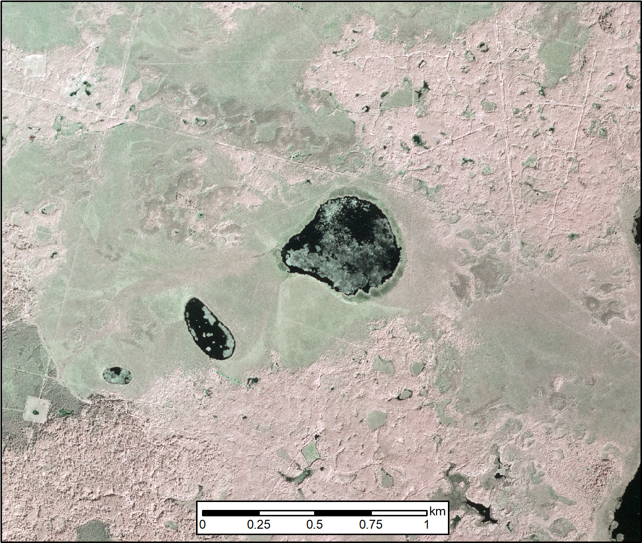
Figure 1. This figure shows open surface waters (black areas) for a location northwest of Fort Saskatchewan, Canada. This image for ABoVE grid ch078v097 was acquired July 9, 2017.
Citation
Kyzivat, E.D., L.C. Smith, L.H. Pitcher, J. Arvesen, T.M. Pavelsky, S.W. Cooley, and S. Topp. 2018. ABoVE: AirSWOT Color-Infrared Imagery Over Alaska and Canada, 2017. ORNL DAAC, Oak Ridge, Tennessee, USA. https://doi.org/10.3334/ORNLDAAC/1643
Table of Contents
- Data Set Overview
- Data Characteristics
- Application and Derivation
- Quality Assessment
- Data Acquisition, Materials, and Methods
- Data Access
- References
Data Set Overview
This dataset contains georeferenced three-band orthomosaics of green, red, and near-infrared (NIR) digital imagery at 1m resolution collected over selected surface waters across Alaska and Canada between July 9 and August 17, 2017. The orthomosaics were generated from individual images collected by a Cirrus Designs Digital Camera System (DCS) mounted on a Beechcraft Super King Air B200 aircraft from approximately 8-11 km altitude. Flights were over the following areas: Saskatchewan River, Saskatoon, Inuvik, Yukon River including Yukon Flats, Sagavanirktok River, Arctic Coastal Plain, Old Crow Flats, Peace-Athabasca Delta, Slave River, Athabasca River, Yellowknife, Great Slave Lake, Mackenzie River and Delta, Daring Lake, and other selected locations. Most locations were imaged twice during two flight campaigns in Canada and Alaska extending roughly SE-NW then NW-SE up to a month apart. The data were georeferenced using 303 ground control points (GCPs) across the study region.
These data are intended to validate surface water extent to aid interpretation of AirSWOT Ka-band radar returns as part of the AirSWOT ABoVE project. The core of AirSWOT is the Ka-band SWOT Phenomenology Airborne Radar (KaSPAR). It collects two swaths of across-track interferometry data - between nadir and 1 km and between 1 km and 5 km, respectively - which can be used to obtain centimeter-level topographic maps of water surfaces. In addition, KaSPAR has an along-track interferometer that can be used to measure the temporal decorrelation of water surfaces, as well as the water radial velocity.
Project: Arctic-Boreal Vulnerability Experiment
The Arctic-Boreal Vulnerability Experiment (ABoVE) is a NASA Terrestrial Ecology Program field campaign based in Alaska and western Canada between 2016 and 2021. Research for ABoVE links field-based, process-level studies with geospatial data products derived from airborne and satellite sensors, providing a foundation for improving the analysis and modeling capabilities needed to understand and predict ecosystem responses and societal implications.
Acknowledgments:
This research received funding from the NASA Terrestrial Ecology Program, grant number NNX17AC60A.
Data Characteristics
Spatial Coverage: Alaska and Canada
ABoVE Reference Locations:
Domain: Core ABoVE
State/territory: Alaska and Canada
Spatial resolution: Data are provided at a 1m x 1m pixel size.
Temporal coverage: 2017-07-09 to 2017-08-17
Temporal resolution: One to three collections per location.
Study Areas (All latitude and longitude given in decimal degrees)
| Site | Westernmost Longitude | Easternmost Longitude | Northernmost Latitude | Southernmost Latitude |
|---|---|---|---|---|
| Alaska and Canada | -149.254166 | -98.64386 | 69.474444 | 46.854333 |
Data file information
There are 330 data files in GeoTIFF (.tif) format, four shapefiles (.shp) provided in .zip folders, and one comma-separated file (.csv) with this dataset. There are also 333 companion files provided in .kmz format.
Table 1. File names and descriptions.
| File names | Descriptions |
|---|---|
| DCS_YYYYMMDD_S##*_ChZZZvZZZ_V#.tif | Orthomosaics (330 files) collected between July 9 and August 17, 2017 in GeoTIFF format (.tif) and clipped to the ABoVE “c-level” grid. |
| DCS_Index.zip | Polygon shapefile that shows the areas of all the orthomosaics. |
| ground_control_points_map.zip | The ground control points (GCPs) used to georeference the orthomosaics, manually digitized from the proprietary Digital Globe EV-WHS image service. The coordinates for the points are found under attributes mapX and mapY. |
| ground_control_points_source.zip | The ground control points (GCPs) as they appeared in the original raster files. The coordinates for the points are found under attributes sourceX and sourceY. |
| ground_control_points_source_transformed.zip | The ground control points (GCPs) after warping transformation. The coordinates for the points are found under attributes Source_tX and Source_tY. |
| ground_control_points.csv | This file is provided for easy georeferencing of the orthomosaics and provides the same data as the shapefiles, however, the variable names (column names) are provided in a longer format. The file provides the ground control points (GCPs), manually digitized from the proprietary Digital Globe EV-WHS image service. The coordinates for the points are found under attributes longitude_map and latitude_map. |
| Companion files | |
| DCS_YYYYMMDD_S##*_ChZZZvZZZ_V#.kmz | The 330 orthomosaic files are provided in .kmz format for viewing in Google Earth. There is one *.kmz file for each *.tif file. |
|
ground_control_points_map.kmz ground_control_points_source.kmz ground_control_points_source_transformed.kmz |
Three of the shapefiles are provided in .kmz format for viewing in Google Earth. |
GeoTIFF Files
File naming syntax:
The .tif files are named DCS_YYYYMMDD_S##*_ChZZZvZZZ.tif
Where:
DCS = Digital Camera System
YYYYMMDD = Acquisition Date
S##* = Flight segment number (###), followed by sub-segment A, B, C, D or X. Letters A-D mean the original flight swath was subdivided before clipping to the ABoVE grid, usually to improve georeferencing quality. Letter X means the swath was never subdivided until clipping to the ABoVE grid.
ChZZZvZZZ= ABoVE grid C horizontal (h) and vertical (v)
Example file name: DCS_20170709_S01X_Ch082v088.tif . The collection date was 20170709, the segment is 1, with sub-segment X, and the extent is within or equal to ABoVE grid C, horizontal index 82, vertical index 88.
Properties of the GeoTIFF Files:
Pixel size= 1m
Three bands: Band 1 (Near-infrared, 760-900 nm), Band 2 (Red, 630-690 nm), Band 3 (Green, 520-600 nm)
Data type= 16-bit signed integers. Data values are scaled to integers in the inclusive range (0, 32767).
No data value= -9999
Note that raster products are georeferenced, orthorectified, but not radiometrically calibrated.
User Note: When displaying rasters, setting the same image stretch to multiple files is recommended when viewing together. Otherwise, the boundaries between individual tiles may be visible, since each tile will have a slightly different stretch.
Spatial and Coordinate System properties of the GeoTIFFS and the shapefile DCS_Index.shp: EPSG Projection (authority: ESRI): 102001
Shapefiles (.shp)
DCS_Index.shp
This is a polygon shapefile that shows the areas of all orthomosaics. The spatial properties of all shapefiles are the same as for the GeoTIFF files described above.
Table 2. Attributes in the shapefile.
| Attribute | Description |
|---|---|
| AboveGrid | ABoVE Grid tile, based on convention |
| OrigRaster | Original raster file name before being clipped to ABoVE grid. All rasters sharing a common “OrigRaster” value were warped to the same affine transformation |
| Date | Image acquisition date |
| GCP_Count | Total number of GCPs contained within raster boundaries. A value of zero indicates either there is no GCP-based warp applied to the raster, or the warp didn’t use any GCPs ontained within the raster boundaries. This column sums to the number of GCPs used for the entire dataset (303) |
| Total_GCP | Total number of GCPs used to warp the original raster file. This number will always be greater than or equal to GCP_count. A value of zero indicates there is no GCP-based warp applied to the raster and the accuracy can be assumed to be less than 5m |
| Avg_diff | Average difference in meters between the GCPs in the final raster file (transformed source coordinate, as found in the GCP shapefiles) and their corresponding “actual” coordinate given in the DigitalGlobe image service. A value of -9999 indicates that there are no GCPs contained within the raster bounds |
| Min_diff | Minimum difference for the above |
| Max_diff | Maximum difference for the above |
Ground Control Point Data
The three shapefiles below and the .csv all file have the same variables and data provided for easy referencing. However, each shapefile will only display the points for the coordinates of two particular variables. The .csv provides all variables with longer variable names.
ground_control_points_map.shp: Provides the GCPs mapX and mapY.
ground_control_points_source.shp: Provides the GCPs sourceX and source_Y.
ground_control_points_source_transformed.shp: Provides the GCPs after warping, source_tx and source_ty.
ground_control_points.csv: This file is provided for easy georeferencing of the orthomosaics. The variable names (column names) are provided in longer format. The file provides the GCPs, manually digitized from the proprietary Digital Globe EV-WHS image service. The coordinates for the points are found under attributes longitude_map and latitude_map.
Table 3. Variables in the GCP data files listed above.
| .CSV variable name | Shape file variable name | Units/format | Description |
|---|---|---|---|
| orig_raster | OrigRaster | Original raster file name before being clipped to ABoVE grid. All rasters sharing a common “original raster” value were warped to the same affine transformation | |
| gcp_number | GCP_number | Sequential ordering of GCPs for each original raster | |
| longitude_orig_raster | sourceX | Decimal degrees | Longitude coordinate in WGS-84 of GCP location as it appeared in original raster file |
| latitude_orig_raster | sourceY | Decimal degrees | Latitude coordinate in WGS-84 of GCP location as it appeared in original raster file |
| longitude_transformed | Source_tX | Decimal degrees | Transformed source: Longitude coordinate in WGS-84 of GCP location after warping transformation. Can be compared to longitude_map to show georeferencing error |
| latitude_transformed | Source_tY | Decimal degrees | Transformed source: Latitude coordinate in WGS-84 of GCP location after warping transformation. Can be compared to latitude_map to show georeferencing error |
| longitude_map | mapX | Decimal degrees | Longitude coordinate in WGS-84 of corresponding GCP location in DigitalGlobe image service, used as “truth” |
| latitude_map | mapY | Decimal degrees | Latitude coordinate in WGS-84 of corresponding GCP location in DigitalGlobe image service, used as “truth” |
| transformed_map_difference | diff | Meters | Euclidian distance, in meters, between transformed source and map points (corresponding “actual” coordinate given in the DigitalGlobe image service-mapX and mapY). Shows final geolocation accuracy for region surrounding this point |
Application and Derivation
These data are intended to validate surface water extent to aid interpretation of AirSWOT Ka-band radar returns as part of the AirSWOT ABoVE project.
Quality Assessment
Geolocation is accurate to ~10 m, with 90% of the files accurate to 20m or less. These accuracies are based on Digital Globe product documentation and analysis of deviation from GCPs after warping. More accurate geolocation was achieved by manually georeferencing the product to Digital Globe imagery.
About one third of the files contain some clouds or cloud shadows. There are some data dropouts due to insufficient pixel correlations between image overlaps. No gap filling has been applied. This effect is most prevalent over clouds, uniform lakes or moving water.
Per standard practice, the camera was integrated with NASA #801 without consideration for circulation of warm, dry air across the camera window which resulted in visual ice formation on the camera during operation. There was noted potential for formation of condensation on camera window. This was not corrected for in data processing.
Data Acquisition, Materials, and Methods
Purpose
These data are intended to validate surface water extent to aid interpretation of AirSWOT Ka-band radar returns as part of the AirSWOT ABoVE project. The core of AirSWOT is the Ka-band SWOT Phenomenology Airborne Radar (KaSPAR). It collects two swaths of across-track interferometry data - between nadir and 1 km and between 1 km and 5 km, respectively - which can be used to obtain centimeter-level topographic maps of water surfaces. In addition, KaSPAR has an along-track interferometer that can be used to measure the temporal decorrelation of water surfaces, as well as the water radial velocity.
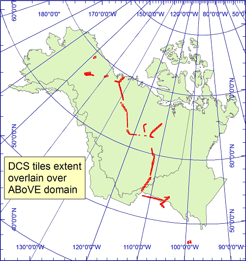
Figure 2. DCS tiles extent in the ABoVE domain.
Image Collection
Digital images were collected using a 16 Megapixel (MP) Cirrus Digital Systems (http://cirrus-designs.com) color infrared camera between July 9 and August 17, 2017. The system records data in green (520-600 nm), red (630-690 nm), and near-infrared (760-900 nm) channels.
The camera was mounted in a NASA #801, a B200 King Air, and enclosed in a box with a 16-inch diameter glass window. For flights prior to July 29, 2017, data were collected with a fixed-length 60 mm lens with a 34° field-of-view. Three different cameras and two different lenses were used. Individual image dimensions were 4072 (width) x 4072 (along-track) before the mosaicking process. For flights after July 29, 2017, data were collected with a fixed-length 80-mm lens with a 25° field-of-view. The auxiliary shutter on the camera malfunctioned, resulting in only partial shutter opening, and vignetting at the top and bottom of each image. This was deemed a mechanical issue that could not be fixed remotely. To minimize vignetting effects for orthomosaic generation, individual images were clipped, resulting in final image dimensions of 4072 (width) x 3472 (along-track) prior to orthomosaic generation. The reduced image size was still sufficient to generate orthomosaics.
Data were recorded through the glass at ~8-11 km altitude over the following areas: Saskatchewan River, Saskatoon, Inuvik, Yukon River including Yukon Flats, Sagavanirktok River, Arctic Coastal Plain, Old Crow Flats, Peace-Athabasca Delta, Slave River, Athabasca River, Yellowknife, Great Slave Lake, Mackenzie River and Delta, Daring Lake, and others not mentioned.
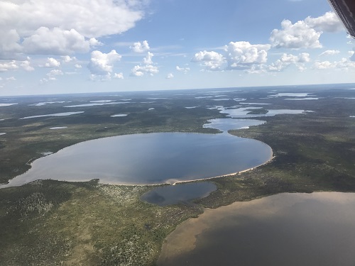
Figure 3. Aerial view of surface water in the study area (photograph by Sarah Cooley).
Image Processing
The orthomosaics were generated from the individual images collected by the DCS (see example in Figure 1). The data were georeferenced using 303 ground control points (GCPs) manually digitized from the Digital Globe EV-WHS web map server. Images were warped in ArcMap 10.6 using a 1st-order polynomial (affine) transformation and the average and root-mean-squared average between the source and map GCPs. Most locations were imaged twice during two flight campaigns in Canada and Alaska extending roughly SE-NW then NW-SE.
The orthomosaics were reprojected to NAD 1983 Canada Albers Equal Area Conic, and resampled to 1m x 1m pixel size. The files are clipped to the ABoVE Standard Reference Grid C (Loboda et al., 2017). The raster products are georeferenced and orthorectified, but not radiometrically calibrated.
Quality Considerations
Image obstruction and striping
Some images were obstructed by clouds and there is no cloud mask provided. Swath sections completely obscured by clouds were removed. In some cases, this resulted in ground areas being imaged only once.
Per standard practice, the camera was integrated with NASA #801 without consideration for circulation of warm, dry air across the camera window which resulted in visual ice formation on the camera during operation. There is noted potential for formation of condensation on camera window. This is not corrected for in data processing.
Most missions were flown during morning hours, where shifting solar conditions resulted in illumination inconsistencies between paths during individual missions. No atmospheric or illumination correction was applied. Striping resulted in some cases where each stripe is the swath width of a particular flight overpass.
Auxiliary shutter malfunction
For flights after July 29, 2017, data were collected with a fixed-length 80-mm lens with a 25-degree field-of-view. The auxiliary shutter on the camera malfunctioned, resulting in only partial shutter opening, and vignetting at the top and bottom of each image. This was deemed a mechanical issue that could not be fixed remotely. To minimize vignetting effects for orthomosaic generation, individual images were clipped, resulting in final image dimensions of 4072 (width) x 3472 (along-track) prior to orthomosaic generation. The reduced image size was still sufficient to generate orthomosaics.
Georeferencing and accuracy assessment
These orthomosaics were produced through Agisoft Photoscan software using positional data from the aircraft (IMU and GPS). The initial product had a geolocation offset ranging from 0-120m between the same ground points imaged on different days. This high uncertainty is due to low or nonexistent side image overlap caused by the linear flight paths, uncertainties in the positional data, the effects of clouds, and the aging camera system used. The initial geolocation accuracy achieved through this method was highly sensitive to small errors in position and was not sufficient for the purposes of comparing to AirSWOT radar images taken concurrently.
This problem was resolved by georeferencing 29 out of the original 38 orthomosaics using 303 ground control points (GCPs) manually digitized from the proprietary Digital Globe EV-WHS image service. This service provides orthorectified imagery with spatial resolution on the order of 1m or better (EnhancedView Web Hosting Service, 2018) . The four operational Digital Globe satellites (Satellite Information, 2018) used as input to the service have a stated 90th percentile geolocation error ranging from 3.0m (GeoEye-1) to 6.5m (Worldview-1). GCPs were chosen as persistent landscape features that could be identified in both the orthomosaics and the Digital Globe image service. Such features included road intersections, and, over the largely unpopulated study area, tree stand boundaries. Images were warped in ArcMap 10.6 using a 1st-order polynomial (affine) transformation, and the average and root-mean-squared average distance between the source and map GCPs was computed. If these numbers differed by more than 20%, the corresponding image was manually split into two or more parts and warp was re-applied, using the corresponding subset of GCPs. These operations were performed on the original orthomosaics using the same geographic coordinate system as the DigitalGlobe service (WGS-84). The orthomosaics were then projected and split to the ABoVE grid, resulting in the 330 files in this archive. If an orthomosaic consistently showed less than a 5m deviation from the DigitalGlobe image, it was assumed to be as accurate as possible, and no GCP-based warping was applied.
After georeferencing, statistics were calculated. 90% of GCPs have a deviation from DigitalGlobe of 13.28 meters (13.28 pixels) or less. Additional statistics on the offset from DigitalGlobe include: min: 0.30m, max: 49.76m, mean: 5.97m, standard deviation: 5.70m. Given that at least 90% of the DigitalGlobe image service has a geolocation error of 6.5m or less [3], the stated horizontal accuracy of our product is at most 19.8m for 90% of the manually georeferenced orthomosaics, with individual accuracies available as shapefile attributes.
Data Access
These data are available through the Oak Ridge National Laboratory (ORNL) Distributed Active Archive Center (DAAC).
ABoVE: AirSWOT Color-Infrared Imagery Over Alaska and Canada, 2017
Contact for Data Center Access Information:
- E-mail: uso@daac.ornl.gov
- Telephone: +1 (865) 241-3952
References
“EnhancedView Web Hosting Service.” 2018 (accessed July 2018). Digital Globe. https://evwhs.digitalglobe.com/myDigitalGlobe/login.
Loboda, T.V., E.E. Hoy, and M.L. Carroll. 2017. ABoVE: Study Domain and Standard Reference Grids. ORNL DAAC, Oak Ridge, Tennessee, USA. https://doi.org/10.3334/ORNLDAAC/1367
“Satellite Information.” 2018 (accessed July 2018). Digital Globe. https://www.digitalglobe.com/resources/satellite-information