Documentation Revision Date: 2020-02-05
Dataset Version: 1
Summary
Whole air samples collected in flasks were analyzed on automated systems at the NOAA Earth System Research Laboratory (ESRL) Global Monitoring Division and the Stable Isotope Laboratory of the Institute of Arctic and Alpine Research (INSTAAR) at the University of Colorado Boulder, which also analyze samples from the NOAA/ESRL Global Greenhouse Gas Reference Network.
There is one data file in comma-separated (.csv) format with results for 51 trace gas analyses and one companion file with laboratory analysis details, one for each trace gas analyte, provided with this dataset.
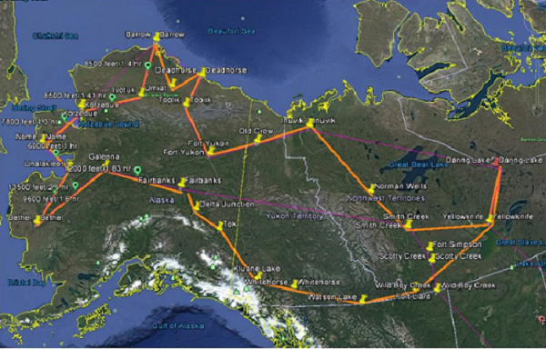
Figure 1. Arctic-CAP flight lines (orange) sample Arctic and boreal regions of Alaska and the Yukon and the Northwest Territories of Canada. Monthly campaigns extended from April through November, capturing the carbon dynamics of the 2017 growing season. Pins mark the locations of the 25 vertical profiles acquired during each monthly campaign. Source: Scientific Aviation, 2019.
Citation
Sweeney, C., K. McKain, B.R. Miller, and S.E. Michel. 2019. ABoVE: Atmospheric Gas Concentrations from Airborne Flasks, Arctic-CAP, 2017. ORNL DAAC, Oak Ridge, Tennessee, USA. https://doi.org/10.3334/ORNLDAAC/1717
Table of Contents
- Dataset Overview
- Data Characteristics
- Application and Derivation
- Quality Assessment
- Data Acquisition, Materials, and Methods
- Data Access
- References
Dataset Overview
This dataset provides atmospheric carbon dioxide (CO2), methane (CH4), carbon monoxide (CO), molecular hydrogen (H2), nitrous oxide (N2O), sulfur hexafluoride (SF6), and other trace gas mole fractions (i.e. "concentrations") from flights over Alaska and the Yukon and Northwest Territories of Canada during the Arctic Carbon Aircraft Profile (Arctic-CAP) monthly sampling campaigns from April-November 2017. The data were derived from laboratory measurements of whole air samples collected by Programmable Flask Packages (PFP) onboard the aircraft. During each of the six monthly campaigns, flights over the Arctic-Boreal Vulnerability Experiment (ABoVE) domain included 25 vertical profiles, from the surface up to 6 km altitude, at locations selected to complement regular long-term vertical profiles, remote sensing data, and ground-based flux tower measurements. Measurements were initiated by the aircraft pilot at predetermined locations within each profile in order to evenly distribute flask sampling points throughout each flight. A total of 408 flask samples were collected during 55 individual flights. The measurements included in this data set are crucial for understanding changes in Arctic carbon cycling and the potential threats posed by thawing of Arctic permafrost.
Whole air samples collected in the PFPs were analyzed on automated systems at the NOAA Earth System Research Laboratory (ESRL) Global Monitoring Division and the Stable Isotope Laboratory of the Institute of Arctic and Alpine Research (INSTAAR) at the University of Colorado Boulder, which also analyze samples from the NOAA/ESRL Global Greenhouse Gas Reference Network.
Project: Arctic-Boreal Vulnerability Experiment
The Arctic-Boreal Vulnerability Experiment (ABoVE) is a NASA Terrestrial Ecology Program field campaign based in Alaska and western Canada between 2016 and 2021. Research for ABoVE links field-based, process-level studies with geospatial data products derived from airborne and satellite sensors, providing a foundation for improving the analysis and modeling capabilities needed to understand and predict ecosystem responses and societal implications.
Related Datasets:
Sweeney, C., J.B. Miller, A. Karion, S.J. Dinardo, and C.E. Miller. 2016. CARVE: L2 Atmospheric Gas Concentrations, Airborne Flasks, Alaska, 2012-2015. ORNL DAAC, Oak Ridge, Tennessee, USA. http://doi.org/10.3334/ORNLDAAC/1404
Sweeney, C., and K. McKain. 2019. ABoVE: Atmospheric Profiles of CO, CO2 and CH4 Concentrations from Arctic-CAP, 2017. ORNL DAAC, Oak Ridge, Tennessee, USA. https://doi.org/10.3334/ORNLDAAC/1658
Acknowledgement:
This research received funding from the NASA Terrestrial Ecology Program, grant number NNX17AC61A.
Data Characteristics
Spatial Coverage: Alaska, USA, and Yukon and the Northwest Territories, Canada
ABoVE Reference Locations:
Domain: Core and extended
State/territory: Alaska, Yukon, Northwest Territories
Grid cells: Ah00v00, Ah00v01, Ah01v01, Ah02v01
Spatial Resolution: Point locations
Temporal Coverage: 2017-04-27 to 2017-11-04
Temporal Resolution: Data were collected in approximately monthly campaigns with 7-8 flight days for each campaign. Measurements were initiated by the aircraft pilot at predetermined locations within each profile in order to evenly distribute flask sampling points throughout each flight.
Study Areas (All latitude and longitude given in decimal degrees)
| Site | Westernmost Longitude | Easternmost Longitude | Northernmost Latitude | Southernmost Latitude |
|---|---|---|---|---|
| Alaska and Canada | -165.4799 | -111.5716 | 71.2712 | 58.0838 |
Data File Information
There is one data file in comma-separated (.csv) format with results for 51 trace gas analyses from 408 flask samples collected during 55 individual flights. These data were collected during the same flights as those in dataset https://doi.org/10.3334/ORNLDAAC/1658. The measured parameters are listed in Table 2. For each measured parameter (parameter_formula in the data file), there are the following attributes: parameter_formula, analysis_group_abbr, analysis_value, and analysis_flag.
Companion files: There is one companion file containing a compressed collection of laboratory analysis details, one file for each trace gas analyte (sample_analysis_per_noaa_instaar_group.zip).
Data Dictionary
Table 1. Parameters and attributes in ABoVE_april-nov_2017_flask_data.csv. Missing values are denoted by -999.99
| Variable | Units/format | Description |
|---|---|---|
|
Sample Descriptors |
||
| sample_year | YYYY | Year of the sample collection |
| sample_month | M | Month of the sample collection- 4, 5, 6 (April, May, and June) |
| sample_day | DD | Day of the sample collection |
| sample_hour | HH | Hour of the sample collection |
| sample_minute | MM | Minute of the sample collection |
| sample_seconds | SS | Seconds of the sample collection |
| sample_id | The sample (flask) container ID. A unique row identifier. [CAUTION: If you open this file in Excel, this column might be converted to a date format by default. “event_number” is also a unique row identifier.] | |
| sample_method | A single-character code that identifies the sample collection method. All values = R | |
| sample_latitude | Decimal degrees | The latitude where the sample was collected (negative (-) numbers indicate samples collected in the southern hemisphere) |
| sample_longitude | Decimal degrees | The longitude where the sample was collected (negative (-) numbers indicate samples collected in the western hemisphere) |
| sample_altitude | m.a.s.l. | The altitude of the sample inlet in meters above sea level (masl) |
| sample_elevation | m | Surface elevation (masl) |
| sample_intake_height | m | Air sample collection height above ground level (magl) |
| event_number | A long integer that uniquely identifies the sampling event | |
|
Analysis Results (54 parameters) |
Column Names: Each parameter is reported as a set of 4 columns. To distinguish columns, the parameter abbreviation (“parameter_formula” and Table 2) is prepended to the base column name. | |
| *_parameter_formula | Trace gas analyte. See Table 2 for full name. | |
| *_analysis_group_abbr | Identifies the group within NOAA, GMD or the Institute of Arctic and Alpine Research (INSTAAR) at the University of Colorado Boulder that made the actual measurement: CCGG: NOAA Carbon Cycle Greenhouse Gases (CCGG) HATS: NOAA Halocarbons and other Atmospheric Trace Species (HATS) SIL: INSTAAR Stable Isotope Laboratory (SIL) |
|
| *_analysis_value | The measured value. Dry air mole fraction or isotopic composition. See Table 2 for units. Missing values are denoted by -999.99 | |
| *_analysis_flag | A three-character field indicating the results of the data rejection and selection process*** |
*** Quality flags:
- valid data = …
- FIL = no data value
- Data should be rejected = anything with a character other than “.” in the first slot such as C… M.., B..
- Preliminary data = …P
Example column names for two parameters:
| BENZ_parameter_formula | Parameter = BENZ |
| BENZ_analysis_group_abbr | Analysis group = HATS |
| BENZ_analysis_value | The measured value. Dry air mole fraction or isotopic composition |
| BENZ_analysis_flag | Flag*** |
| sf6_HATS_parameter_formula | Parameter = sf6 [Note that sf6 was analyzed by both HATS and CCGG groups. Thus, the “analysis_group_abbr” was also prepended to the base column name.] |
| sf6_HATS_analysis_group_abbr | Analysis group = HATS |
| sf6_HATS_analysis_value | The measured value. Dry air mole fraction or isotopic composition |
| sf6_HATS_analysis_flag | Flag*** |
Table 2. Parameters (trace gases) in the data file, in the order as they appear in the file.
| Parameter abbreviation | Parameter name or formula | Units |
|---|---|---|
| BENZ | benzene (C6H6) | parts per trillion (ppt) |
| BRFM | bromoform (CHBr3) | ppt |
| C2F6 | hexafluoroethane (CF3CF3) | ppt |
| C2H2 | ethyne (acetylene; C2H2) | ppt |
| C2H6 | ethane (C2H6) | ppt |
| C3H8 | propane (C3H8) | ppt |
| CCL4 | carbon tetrachloride (tetrachloromethane; CCl4) | ppt |
| CF4 | carbon tetraflouride (tetrafluoromethane; CF4) | ppt |
| CH3I | methyl iodide (CH3I) | ppt |
| CH4 | methane (CH4) | parts per billion (ppb) |
| CH4C13 | methane-isotopic composition C13 | |
| CHLF | chloroform (CHCl3) | ppt |
| CO | carbon monoxide (CO) | ppb |
| CO2 | carbon dioxide (CO2) | parts per million (ppm) |
| DIBR | dibromomethane (CH2Br2) | ppt |
| DICL | dichloromethane (CH2Cl2) | ppt |
| F113 | CFC-113 (CCl2FCClF2) | ppt |
| F115 | chloropentafluoroethane (CFC-115; (CClF2CF3)) | ppt |
| F11B | CFC-11; (ion 103; CCl3F) | ppt |
| F125 | HFC-125 (CHF2CF3) | ppt |
| F13 | chlorotrifluoromethane (CFC-13; (CClF3)) | ppt |
| F134A | HFC-134a (CH2FCF3) | ppt |
| F142B | HCFC-142b (CH3CF2Cl) | ppt |
| F143A | HFC-143a (CH3CF3) | ppt |
| F152A | HFC-152a (CH3CHF2) | ppt |
| F227E | HFC-227ea (CF3CHFCF3) | ppt |
| F23 | trifluoromethane (HFC-23; (CHF3)) | ppt |
| F236FA | HFC-236fa (CF3CH2CF3) | ppt |
| F32 | difluoromethane (HFC-32; (CH2F2)) | ppt |
| F365M | HFC-365mfc (CH3CF2CH2CF3) | ppt |
| FC12 | dichlorodifluoromethane (CFC-12; (CCl2F2)) | ppt |
| H1211 | bromochlorodifluoromethane (halon 1211; CBrClF2) | ppt |
| H1301 | bromotrifluoromethane (halon 1301; CF3Br) | ppt |
| H2 | hydrogen (H2) | ppb |
| H2402 | dibromotetrafluoroethane (halon 2402; CBrF2CBrF2) | ppt |
| HF133a | HCFC-133a (CH2ClCF3) | ppt |
| HF22 | HCFC-22 (CHF2Cl) | ppt |
| IC4H10 | i-butane (i-C4H10) | ppt |
| IC5H12 | i-pentane (i-C5H12) | ppt |
| MCFA | methyl chloroform (ion 97; CH3CCl3) | ppt |
| MEBR | methyl bromide (CH3Br) | ppt |
| MECL | methyl chloride (CH3Cl) | ppt |
| N2O | nitrous oxide (N2O) | ppb |
| NC4H10 | n-butane (n-C4H10) | ppt |
| NC5H12 | n-pentane (n-C5H12) | ppt |
| NC6H14 | n-hexane (n-C6H14) | ppt |
| OCS | carbonyl sulfide (COS) | ppt |
| P218 | perfluoropropane (C3F8) | ppt |
| PCE | tetrachloroethylene (C2Cl4) | ppt |
| SF6 (CCGG and HATS) | sulfur hexafluoride (SF6) | ppt |
| SO2F2 | sulfuryl fluoride (SO2F2) | ppt |
Application and Derivation
Large changes in surface air temperature, sea ice cover and permafrost in the Arctic Boreal Ecosystems (ABE) are likely to have significant impact on the critical ecosystem services and the human societies that are dependent on the ABE. In order to predict the outcome of continued change to the climate system in the ABE, it is necessary to understand the vulnerabilities of the underlying ABE ecosystems by understanding what processes drive both spatial variability and interannual variability.
These data contribute to our understanding and predictive capabilities for modeling the land-atmospheric exchange of CO2 and CH4 to better understand the feedbacks that these greenhouse gases will have on the ABE.
Quality Assessment
Table 3. Repeatability of gas detection was determined as 1 standard deviation of ~20 aliquots of natural air measured from a standard cylinder.
| Gas | Average Repeatability |
|---|---|
| CO | UV Resonance fluorescence: +/- 0.4 ppb (Gerbig et al., 1999) |
| CO2 | +/- 0.03 ppm (Conway et al., 1994) |
| CH4 | +/- 1.2 ppb (Dlugokencky et al., 1994) |
| H2 | +/- 0.4 ppb (Novelli et al., 1999) |
| N2O | +/- 0.26 ppb (Dlugokencky et al., 2009) |
| SF6 | +/- 0.03 ppt (Dlugokencky et al., 2009) |
Data Acquisition, Materials, and Methods
The Arctic Carbon Aircraft Profile (Arctic-CAP) project was designed to measure vertical profiles of atmospheric CO2, CH4, and CO concentrations to capture the spatial and temporal dynamics of the northern high latitude carbon cycle as part of the Arctic-Boreal Vulnerability Experiment (ABoVE) (Miller et al., 2019).
Arctic-CAP flights consisted of vertical profile maneuvers from near the surface to 6 km altitude around the ABoVE domain each month. Profile locations were selected to complement regular long-term vertical profiles, remote sensing data, and ground-based flux tower measurements. These data spatially link the regular vertical profiles obtained at Poker Flats, AK and East Trout Lake, SK as part of the ESRL/GMD Aircraft Program (https://www.esrl.noaa.gov/gmd/ccgg/aircraft/). These measurements were complemented by additional vertical profiles that were acquired at altitudes up to 14 km by the NASA DC-8 in August (Active Sensing of CO2 Emissions over Nights, Days, & Seasons [ASCENDS], https://www-air.larc.nasa.gov/missions/ascends/index.html) and October (Atmospheric Tomography Mission [AToM], Wofsy et al. (2018)). Six campaigns were flown from April to early November in 2017 with instrumentation aboard a Mooney Ovation 3 M20R (N617DH, Scientific Aviation).
The Arctic-CAP aircraft carried an atmospheric sampling payload consisting of a continuous greenhouse gas analyzer ( https://doi.org/10.3334/ORNLDAAC/1658) and a flask sampling system. This data set includes measurements from discrete air samples captured by the flask sampling system. The flask sampling system consisted of a Programmable Flask Package (PFP) and Programmable Compressor Package (PCP), which are used routinely on aircraft as part of the NOAA/ESRL Global Monitoring Division’s Carbon Cycle and Greenhouse Gases network (Sweeney et al., 2015). The flask sampling strategy on Arctic-CAP involved acquiring whole-air samples evenly distributed throughout each flight. The measurements made on the whole-air flask samples are described in Table 2.
Gas detection
- Quantities of CO2 in flask air samples were detected using a non-dispersive infrared analyzer and reported in parts per million (ppm). Because detector response is non-linear in the range of atmospheric levels, ambient samples are bracketed during analysis by a set of reference standards used to calibrate detector response.
- CH4 was isolated from constituent gases through gas chromatography and quantified with flame ionization detection. Measurements are reported in parts per billion (ppb).
- CO was isolated from constituent gases with gas chromatography and detected by resonance fluorescence at ~150 nm, or by reaction with HgO to produce mercury and detection through Hg resonance absorption and reported in ppb.
- H2 was isolated using gas chromatography, reacted with HgO, and detected through Hg resonance absorption. H2 quantities are reported in ppb.
- The N2O and SF6 sample components were isolated using gas chromatography and quantified with electron capture detection. N2O and SF6 are reported in ppb and parts per trillion (ppt), respectively.
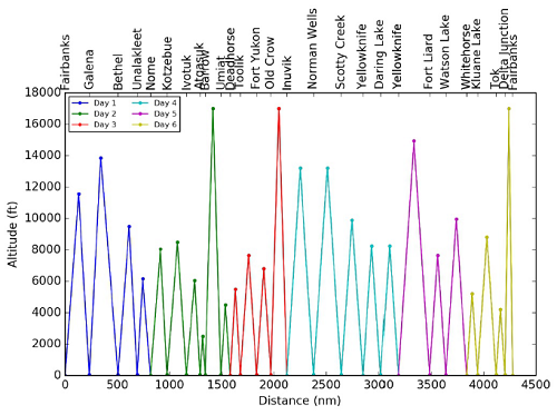
Figure 2. For each campaign, vertical profiles were flown at each of the ~25 locations listed across the top of this figure. These locations are shown on Figure 1. Nominally, the campaign would require six flying days to complete all profiles.
Data Access
These data are available through the Oak Ridge National Laboratory (ORNL) Distributed Active Archive Center (DAAC).
ABoVE: Atmospheric Gas Concentrations from Airborne Flasks, Arctic-CAP, 2017
Contact for Data Center Access Information:
- E-mail: uso@daac.ornl.gov
- Telephone: +1 (865) 241-3952
References
Conway, T.J., P.P. Tans, L.S. Waterman, K.W. Thoning, D.R. Kitzis, K.A. Masarie, and N. Zhang. (1994). Evidence for interannual variability of the carbon cycle from the National Oceanic and Atmospheric Administration/Climate Monitoring and Diagnostics Laboratory Global Air Sampling Network, J. Geophys. Res., 99, 22,831–22,855. https://doi.org/10.1029/94JD01951
Dlugokencky, E.J., L.Bruhwiler, J.W.C. White, L.K. Emmons, P.C. Novelli. S.A. Montzka, K.A. Masarie, P.M. Lang, A.M. Crotwell, J.B. Miller, and L.V. Gatti. (2009). Observational constraints on recent increases in the atmospheric CH4 burden, Geophys. Res. Lett., 36, L18803. https://doi.org/10.1029/2009GL039780
Dlugokencky, E.J., L.P. Steele, P.M. Lang, K.A. Masarie (1994). The growth rate and distribution of atmospheric methane, J. Geophys. Res., 99, 17,021–17,043.https://doi.org/10.1029/94JD01245
Gerbig, C., S. Schmitgen, D. Kley, A. Volz-Thomas, K. Dewey, D. Haaks (1999). An improved fast-response vacuum-UV resonance fluorescence CO instrument, J. Geophys. Res. 104, 1699 –1704.https://doi.org/10.1029/1998JD100031
Miller, C.E., P. Griffith, S. Goetz, E. Hoy, N. Pinto, I. Mccubbin, A.K. Thorpe, M.M. Hofton, D.J. Hodkinson, and C. Hansen, J. Woods, E.K. Larsen, E.S. Lasischke, and H. Margolis. 2019. An overview of ABoVE airborne campaign data acquisitions and science opportunities. Environmental Research Letters. https://doi.org/10.1088/1748-9326/ab0d44
Novelli, P.C., P.M. Lang, K.A. Masarie, D.F. Hurst, R. Myers, J.W. Elkins (1999). Molecular hydrogen in the troposphere: Global distribution and budget, J. Geophys. Res. 104, 30,427-30,444.https://doi.org/10.1029/1999JD900788
Scientific Aviation. 2019. Company Website (http://www.scientificaviation.com/). Arctic-CAP flight lines image: http://www.scientificaviation.com/wp-content/uploads/2019/01/cropped-Above_Loop.jpg Accessed 20190409.
Sweeney, C., A. Karion, S. Wolter, T. Newberger, D. Guenther, J.A. Higgs, A.E. Andrews, P.M. Lang, D. Neff, E. Dlugokencky, and J.B. Miller. 2015. Seasonal climatology of CO2 across North America from aircraft measurements in the NOAA/ESRL Global Greenhouse Gas Reference Network. Journal of Geophysical Research: Atmospheres, 120(10), pp.5155-5190. https://doi.org/10.1002/2014JD022591
Sweeney, C., and K. McKain. 2019. ABoVE: Atmospheric Profiles of CO, CO2 and CH4 Concentrations from Arctic-CAP, 2017. ORNL DAAC, Oak Ridge, Tennessee, USA. https://doi.org/10.3334/ORNLDAAC/1658
Wofsy, S.C., S. Afshar, H.M. Allen, E. Apel, E.C. Asher, B. Barletta, J. Bent, H. Bian, B.C. Biggs, D.R. Blake, N. Blake, I. Bourgeois, C.A. Brock, W.H. Brune, J.W. Budney, T.P. Bui, A. Butler, P. Campuzano-Jost, C.S. Chang, M. Chin, R. Commane, G. Correa, J.D. Crounse, P. D. Cullis, B.C. Daube, D.A. Day, J.M. Dean-Day, J.E. Dibb, J.P. DiGangi, G.S. Diskin, M. Dollner, J.W. Elkins, F. Erdesz, A.M. Fiore, C.M. Flynn, K. Froyd, D.W. Gesler, S.R. Hall, T.F. Hanisco, R.A. Hannun, A.J. Hills, E.J. Hintsa, A. Hoffman, R.S. Hornbrook, L.G. Huey, S. Hughes, J.L. Jimenez, B.J. Johnson, J.M. Katich, R.F. Keeling, M.J. Kim, A. Kupc, L.R. Lait, J.-F. Lamarque, J. Liu, K. McKain, R.J. Mclaughlin, S. Meinardi, D.O. Miller, S.A. Montzka, F.L. Moore, E.J. Morgan, D.M. Murphy, L.T. Murray, B.A. Nault, J.A. Neuman, P.A. Newman, J.M. Nicely, X. Pan, W. Paplawsky, J. Peischl, M.J. Prather, D.J. Price, E. Ray, J.M. Reeves, M. Richardson, A.W. Rollins, K.H. Rosenlof, T.B. Ryerson, E. Scheuer, G.P. Schill, J.C. Schroder, J.P. Schwarz, J.M. St.Clair, S.D. Steenrod, B.B. Stephens, S.A. Strode, C. Sweeney, D. Tanner, A.P. Teng, A.B. Thames, C.R. Thompson, K. Ullmann, P.R. Veres, N. Vieznor, N.L. Wagner, A. Watt, R. Weber, B. Weinzierl, P. Wennberg, C.J. Williamson, J.C. Wilson, G.M. Wolfe, C.T. Woods, and L.H. Zeng. 2018. ATom: Merged Atmospheric Chemistry, Trace Gases, and Aerosols. ORNL DAAC, Oak Ridge, Tennessee, USA. https://doi.org/10.3334/ORNLDAAC/1581