Documentation Revision Date: 2020-03-02
Dataset Version: 1
Summary
Green, red, and near-infrared (NIR) digital imagery was collected with a Cirrus Designs Digital Camera System (DCS) mounted on a B200 aircraft from approximately 8-11 km altitude over the following areas: Saskatchewan River, Saskatoon, Inuvik, Yukon River including Yukon Flats, Sagavanirktok River, Arctic Coastal Plain, Old Crow Flats, Peace-Athabasca Delta, Slave River, Athabasca River, Yellowknife, Great Slave Lake, Mackenzie River and Delta, Daring Lake, and other selected locations. Most locations were imaged twice during two flight campaigns in Canada and Alaska extending roughly SE-NW then NW-SE up to a month apart.
Water masks are provided for 330 individual ABoVE grid cells (ChxxCvxx) in three data file formats: 1-m resolution GeoTIFF (*.tif) files, as converted to Shapefiles (*.shp), and as converted to Google Earth format (*.kml). Shapefiles are provided in compressed format (*.zip). There are four value-added water mask shapefiles (*.shp) produced by combining all of the shapefiles and with additional processing and filtering of water bodies. These four files are also provided in Google Earth (*.kml) format. Characteristics of the original orthomosaic images (coverage, quality and cloud flags, georeferencing data) and image processing metadata are provided in a comma-separated (.csv) file, as converted to a Shapefile (.shp), and as converted to Google Earth format (.kml). There are 1,001 data files in total.
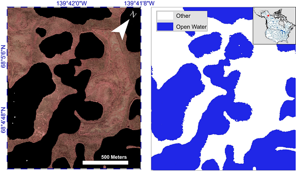
Figure 1: Example of color-infrared imagery shown alongside the corresponding semi-automated open water classification, location: Old Crow Flats, Alaska.
Citation
Kyzivat, E.D., L.C. Smith, L.H. Pitcher, J.V. Fayne, S.W. Cooley, M.G. Cooper, S. Topp, T. Langhorst, M.E. Harlan, C.J. Gleason, and T.M. Pavelsky. 2019. ABoVE: AirSWOT Water Masks from Color-Infrared Imagery over Alaska and Canada, 2017. ORNL DAAC, Oak Ridge, Tennessee, USA. https://doi.org/10.3334/ORNLDAAC/1707
Table of Contents
- Dataset Overview
- Data Characteristics
- Application and Derivation
- Quality Assessment
- Data Acquisition, Materials, and Methods
- Data Access
- References
Dataset Overview
This dataset provides a conservative open water mask for future water surface elevation (WSE) extraction from the co-registered AirSWOT Ka-band interferometry data, and high-resolution (1 m) water body distribution maps for water bodies greater than 40 m2 along the NASA Arctic-Boreal Vulnerability Experiment (ABoVE) foundational flight lines. The masks and maps were derived from georeferenced three-band orthomosaics generated from individual images collected during the flights and a semi-automated water classification algorithm based on the Normalized Difference Water Index (NDWI). In total, 3,167 km2 of open water were mapped from 23,380 km2 of flight lines spanning 23 degrees of latitude. Detected water body sizes range from 40 m2 to 15 km2. The image tiles were georeferenced using manually selected ground control points (GCPs). Comparison with manually digitized open water boundaries yields an overall open-water classification accuracy of 98.0%.
Green, red, and near-infrared (NIR) digital imagery was collected with a Cirrus Designs Digital Camera System (DCS) mounted on a B200 aircraft from approximately 8-11 km altitude over the following areas: Saskatchewan River, Saskatoon, Inuvik, Yukon River including Yukon Flats, Sagavanirktok River, Arctic Coastal Plain, Old Crow Flats, Peace-Athabasca Delta, Slave River, Athabasca River, Yellowknife, Great Slave Lake, Mackenzie River and Delta, Daring Lake, and other selected locations. Most locations were imaged twice during two flight campaigns in Canada and Alaska extending roughly SE-NW then NW-SE up to a month apart.
Project: Arctic-Boreal Vulnerability Experiment
The Arctic-Boreal Vulnerability Experiment (ABoVE) is a NASA Terrestrial Ecology Program field campaign based in Alaska and western Canada between 2016 and 2021. Research for ABoVE links field-based, process-level studies with geospatial data products derived from airborne and satellite sensors, providing a foundation for improving the analysis and modeling capabilities needed to understand and predict ecosystem responses and societal implications.
Related Publications:
Kyzivat, E.D., L.C. Smith, L.H. Pitcher, J.V. Fayne, S.W. Cooley, M.G. Cooper, S. Topp, T. Langhorst, M. Harlan, C. Horvat, C. J. Gleason, and T.M. Pavelsky. A High-Resolution Airborne Color-Infrared Camera Water Mask for the NASA ABoVE Campaign. Remote Sensing, 2019, 11(18), 2163. https://doi.org/10.3390/rs11182163
Related Datasets:
Kyzivat, E.D., L.C. Smith, L.H. Pitcher, J. Arvesen, T.M. Pavelsky, S.W. Cooley, and S. Topp. 2018. ABoVE: AirSWOT Color-Infrared Imagery Over Alaska and Canada, 2017. ORNL DAAC, Oak Ridge, Tennessee, USA. https://doi.org/10.3334/ORNLDAAC/1643
Fayne, J.V., L.C. Smith, L.H. Pitcher, and T.M. Pavelsky. 2019. ABoVE: AirSWOT Ka-band Radar over Surface Waters of Alaska and Canada, 2017. ORNL DAAC, Oak Ridge, Tennessee, USA. https://doi.org/10.3334/ORNLDAAC/1646
Pitcher, L.H., L.C. Smith, T.M. Pavelsky, J.V. Fayne, S.W. Cooley, E.H. Altenau, D.K. Moller, and J. Arvesen. 2019. ABoVE: AirSWOT Radar, Orthomosaic, and Water Masks, Yukon Flats Basin, Alaska, 2015. ORNL DAAC, Oak Ridge, Tennessee, USA. https://doi.org/10.3334/ORNLDAAC/1655
Acknowledgements:
This work was supported by NASA Terrestrial Ecology Program Grant NNX17AC60A, NASA Surface Water and Ocean Topography mission grant number NNX16AH83G, American Meteorological Society Graduate Fellowship, NASA Rhode Island Space Grant Consortium Graduate Fellowship.
Data Characteristics
Spatial Coverage: Alaska, North Dakota, USA. Alberta, Manitoba, Saskatchewan, and the Yukon and the Northwest Territories of Canada
ABoVE Reference Locations:
Domain: Core ABoVE
State/territory: Alaska and Yukon and Northwest Territories of Canada
Grid cells: The data cover 330 grid cells in the range Ch44Cv29 – Ch106v129. Most data are in cells Ch061-Ch093.
These cells are in the large grids Ah1Av0, Ah2Av1, Ah2Av2, and Ah2Av3. Data are in most, but not every cell in this range.
The cells are provided in the data files WC_Index.csv and WC_Index.shp.
Spatial Resolution: 1 m
Temporal Coverage: Flights conducted from 2017-07-09 to 2017-08-17
Temporal Resolution: One to three collections per location
Study Areas (All latitude and longitude given in decimal degrees)
| Site | Westernmost Longitude | Easternmost Longitude | Northernmost Latitude | Southernmost Latitude |
|---|---|---|---|---|
| Alaska and Canada | -152.184966 | -98.63756 | 76.27557 | 43.2700 |
Data File Information
Water masks are provided for 330 ABoVE grid cells (ChxxCvxx) in three data file formats: 1-m resolution GeoTIFF (*.tif) files, as converted to Shapefiles (*.shp), and as converted to Google Earth format (*.kml). Shapefiles are provided in compressed format (*.zip).
There are four value-added water mask shapefiles (*.shp) produced by combining all of the shapefiles and with additional processing and filtering of water bodies. These four files are also provided in Google Earth (*.kml) format.
Characteristics of the original orthomosaic images (coverage, quality and cloud flags, georeferencing data) and image processing metadata are provided in a comma-separated (.csv) file, as converted to a Shapefile (.shp), and as converted to Google Earth format (.kml).
There are 1,001 data files in total.
Table 1. File descriptions. Note that all shapefiles (.shp data files and .shp companion files) are provided in compressed format (.zip).
| File Names | Descriptions |
|---|---|
| Water Mask Data | |
| WC_YYYYMMDD_S0XX*_ChZZZvZZZ_V1.tif | 330 water mask rasters (.tif format) derived from orthomosaics |
| WC_YYYYMMDD_S0XX*_ChZZZvZZZ_V1.shp | 330 water masks (.tifs) were converted to shapefiles (.shp) with smoothed edges. Empty files indicate no water present in the image. Provided in compressed format (.zip). |
| WC_YYYYMMDD_S0XX*_ChZZZvZZZ_V1.kml | 330 water masks (.tiffs) converted Google Earth format (.kml) with smoothed edges. Empty files indicate no water present in the image. |
| Combined and Filtered Mask Data | |
| WC_all_water.shp | Combined shapefile of all water masks, excluding repeat areas. Provided in compressed format (.zip). |
| WC_all_water.kml | Above file converted to Google Earth format (.kml). |
| WC_no_rivers.shp | Combined shapefile of all water masks, with river networks and partial water bodies manually removed. Provided in compressed format (.zip). |
| WC_no_rivers.kml | Above file converted to Google Earth format (.kml). |
| WC_fused_hydroLakes.shp | Combined shapefile of all water masks, with river networks and partial water bodies removed or fused to their corresponding HydroLAKES water body (Messager et al., 2016) if available. Provided in compressed format (.zip). |
| WC_fused_hydroLakes.kml | Above file converted to Google Earth format (.kml). |
| WC_fused_hydroLakes_buf_10_sum.shp | Combined shapefile of all water masks, with a 10-m buffer applied and adjoining water bodies dissolved into one, so each feature represents a single water body. Provided in compressed format (.zip). |
| WC_fused_hydroLakes_buf_10_sum.kml | Above file converted to Google Earth format (.kml). |
| Image Processing Metadata | |
| WC_Index.csv | A comma-separated file with image coverage, quality and cloud flags, and georeferencing data. |
| WC_index.shp | A shapefile with the above information. Provided in compressed format (.zip). |
| WC_index.kml | Above file converted to Google Earth format (.kml). |
Naming Conventions for Water Mask Data Files
The extent (.ext) may be .tif, .shp (.zip), or .kml
Files are named as WC_YYYYMMDD_S0XX*_ChZZZvZZZ_V1.ext
Where:
WC = Water classification
YYYYMMDD = Acquisition Date
S0XX* = Flight segment number, followed by sub-segment A, B, C, D or X. Letters A-D mean the original flight swath was subdivided before clipping to the ABoVE grid, usually to improve georeferencing quality. Letter X means the swath was never subdivided until clipping to the ABoVE grid.
ChZZZvZZZ= ABoVE grid C horizontal index (h) and vertical index (v)
V1= version1
Example file name: WC_20170709_S01X_Ch082v088_V1.tif
The collection date was 20170709, the segment is 1, with sub-segment X, and the extent is within or equal to ABoVE grid C, horizontal index 82, vertical index 88.
Properties of the GeoTIFF Files:
Pixel size = 1 m
Number of bands = 1
Data type = 8-bit signed integers
Pixel values = 1 (open water) or 0 (other)
No data value = -99
Coordinate Reference System: EPSG 102001
Properties of the Shapefiles:
Coordinate Reference System: EPSG 102001
Water Mask Shapefiles (330 files)
These files have one (1) attribute, where a value of 1 indicates that the polygon is open water.
Combined and Filtered Water Mask Shapefiles (4 files)
Table 2. Attributes in the four water mask shapefiles
| Attribute Description | Attribute Description |
|---|---|
| Area | Water body area (square km) |
| Perimeter | Water body perimeter (km) |
| Centroid_x | Longitude of region centroid (decimal degrees, NAD83) |
| Centroid_y | Latitude of region centroid (decimal degrees, NAD83) |
| Region4 | Region code (Table 4 below) |
| Category4 | Hydrologic landscape category (Table 5 below) |
| Area_sum | Sum of areas of enclosed open water bodies (not the area of the shape, which is buffered). Only in the file WC_fused_hydroLakes_buf_10_sum.shp |
| Join_count | Number of enclosed open water bodies that were aggregated to produce feature. Only in the file WC_fused_hydroLakes_buf_10_sum.shp |
Table 3. Attributes in the three WC_Index files (.csv, .shp, .kml). The no data/missing data value is -9999.
| Attribute Description | Attribute Description |
|---|---|
| Filename | Filename of associated image. To obtain the filename of water mask in this archive, replace “DCS” with “WC”. |
| AboveGrid | ABoVE Grid tile |
| OrigRaster | Original raster file name before being clipped to ABoVE grid. All rasters sharing a common “OrigRaster” value were warped to the same affine transformation |
| Date_acq | Image acquisition date |
| GCP_Count | Total number of GCPs contained within raster boundaries. A value of zero indicates either there is no GCP-based warp applied to the raster, or the warp didn’t use any GCPs contained within the raster boundaries. This column sums to the number of GCPs used for the entire dataset (303). |
| Total_GCP | Total number of GCPs used to warp the original raster file. This number will always be greater than or equal to GCP_count. A value of zero indicates there is no GCP-based warp applied to the raster and the accuracy can be assumed to be less than 5m. |
| Avg_diff | Average difference in meters between the GCPs in the final raster file (transformed source coordinate, as found in the GCP shapefiles) and their corresponding “actual” coordinate given in the DigitalGlobe image service. A value of -9999 indicates that there are no GCPs contained within the raster bounds. |
| Min_diff | Minimum difference for the above |
| Min_diff | Maximum difference for the above |
| Area | Area of imaged region, in square km |
| Quality | 0=pervasive classification issues, 0.5= some issues, 1=no evident issues |
| Clouds | 1= clouds or cloud shadows, 0=otherwise |
| Haze | 1= haze, 0=otherwise |
| RiverDomin | River dominance: 1=the flight line predominately follows a river, 0=otherwise |
| Region4 | Region code (see below) |
| Category4 | Physiographic category (see below) |
| WaterIndex | Water index used as basis for classification: either NDWI or the near-infrared band (NIR) |
Table 4. Geographic regions used for analysis
| Region code | Acronym | Region name |
| 2 | SAG | Sagavanirktok River |
| 3 | YFB | Yukon Flats Basin |
| 4 | OCF | Old Crow Flats |
| 5 | MRD | Mackenzie River Delta |
| 6 | MRV | Mackenzie River Valley |
| 7 | CSM | Canadian Shield Margin |
| 8 | CSH | Canadian Shield |
| 9 | SLR | Slave River |
| 10 | PAD | Peace-Athabasca Delta |
| 11 | ATR | Athabasca River |
| 12 | PPN | Prairie Potholes North |
| 13 | PPS | Prairie Potholes South |
| 14 | TKP | Tuktoyaktuk Peninsula |
Table 5. Physiographic categories used for analysis
| Category code | Category |
| 1 | Prairie pothole region |
| 2 | Canadian Shield |
| 3 | Thermokarst |
| 4 | Arctic-boreal wetlands |
| 5 | Lowland river valleys |
Application and Derivation
The dataset provides a conservative open water pixel mask for future water surface elevation (WSE) extraction from the co-registered AirSWOT Ka-band interferometry dataset.
Quality Assessment
The classifier worked best on uniform images free from clouds, haze, shadows, and mosaicking artifacts. False positives arose from roads, buildings, shadows from clouds, tree and terrain, and dark-colored agricultural fields. False negatives arose from the reflective properties of highly turbid water, especially if occurring within the same scene as clear water. Classification errors were assessed by manually digitizing validation water bodies and computing a confusion matrix. Statistics were assessed on a per-pixel and per-object basis between this manual water mask and the output from the classifier. The overall accuracy is 98.0%, with user’s and producer’s accuracies of 87.1% and 94.0%, respectively, and a kappa coefficient of 89.3%. Results were visually compared to shoreline maps derived from in-situ GPS surveys to provide an extra level of certainty. In most cases, the walked shorelines were inland of or equal to the classified shorelines, implying that the classifier was conservative in selecting water (Kyzivat et al., 2019).
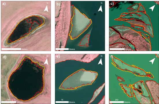
Figure 2. Ground validation sites used for comparison with the classification. Walked shorelines are plotted in gold and classified shorelines in red (only outlines are shown for visual clarity). (a, d) Sandbar islands in the North Saskatchewan River near Saskatoon, SK (shoreline survey less than 4.5 hours after AirSWOT flight); (b, e) Lake in the Canadian Shield East near Yellowknife, NWT (survey less than 21 hours before flight); (c, f) Sandbar islands in the Yukon River in Yukon Flats Basin (survey less than 73 and 30 hours after flight, respectively).
Data Acquisition, Materials, and Methods
2017 AirSWOT Campaign
AirSWOT deployments as part of the 2017 ABoVE campaign occurred in two legs. Northbound flights from North Dakota to the North Slope, Alaska occurred between July 9-21, 2017. Southbound sorties from August 6-17, 2017. The overlapping flight lines were chosen to cover key field stations and to provide data to support model-, field-, and satellite-based studies. Imagery was acquired on 15 days within this period (Table 6). The areas imaged by AirSWOT include the Yukon Flats Basin (YFB), a floodplain wetland environment along the Yukon River, near Ft. Yukon, AK, the Mackenzie River Delta (MRD), NWT, Canada, Precambrian Canadian Shield lakes (CSH) near Yellowknife, NWT, the Peace-Athabasca Delta (PAD), the largest inland delta in North America, AB, and prairie pothole and agricultural lakes, SK, ND.
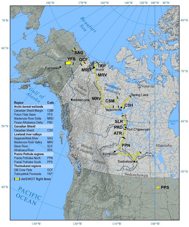
Figure 3. Study area map showing 13 sub-regions organized into five categories. Flight lines followed the foundational flight lines for the 2017 ABoVE airborne campaign and covered some of the most water-rich regions of the world, across climate and permafrost gradients (Kyzivat et al., 2019).
Table 6. Acquisition dates and key to acronyms for study areas, in order of northwest to southeast (Kyzivat et al., 2019).
| Region | Site Code | Category | Area (km2) | Northbound Flight(s) | Southbound Flight(s) |
|---|---|---|---|---|---|
| Sagavanirktok River | SAG | Lowland river valley | 309 | July 19 | - |
| Yukon Flats Basin | YFB | Wetland | 4,601 | July 17, 20, 21 | August 6, 7 |
| Old Crow Flats | OCF | Thermokarst | 653 | - | August 7 |
| Mackenzie River Delta | MRD | Wetland | 409 | July 16 | August 7 |
| Tuktoyaktuk Peninsula | TKP | Thermokarst | 3,748 | July 16 | August 9 |
| Mackenzie River Valley | MRV | Lowland river valley | 814 | - | August 9 |
| Canadian Shield Margin | CSM | Wetland | 2,183 | July 15 | August 9, 12 |
| Canadian Shield | CSH | Shield | 878 | - | August 12, 15 |
| Slave River | SLR | Lowland river valley | 1,509 | - | August 13 |
| Peace-Athabasca Delta | PAD | Wetland | 1,011 | - | August 13 |
| Athabasca River | ATR | Lowland river valley | 5,289 | July 9 | August 13 |
| Prairie Potholes North | PPN | Pothole, Lowland river valley1 | 880 | July 9 | August 16-17 |
| Prairie Potholes South | PPS | Pothole | 1,095 | - | August 17 |
| All regions | - | - | 23,380 | - | - |
Image Acquisition
Green, red, and near-infrared (NIR) digital imagery was collected with a Cirrus Designs Digital Camera System (DCS) mounted on a B200 aircraft from approximately 8-11 km altitude. For flights prior to July 29, 2017, data were collected with a fixed-length 60 mm lens with a 34-degree field-of-view. Three different cameras and two different lenses were used. For flights after July 29, 2017, data were collected with a fixed-length 80 mm lens with a 25-degree field-of-view. Most locations were imaged twice during two flight campaigns in Canada and Alaska extending roughly SE-NW then NW-SE.
Raw images were digitally stitched and orthorectified in Agisoft PhotoScan if they had less than 50% cloud cover. This step resulted in 38 orthomosaics at 1 m resolution, which were used for further processing. The data were georeferenced using 303 ground control points (GCPs) manually digitized from the Digital Globe EV-WHS web map server. Images were warped in ArcMap 10.6 using a 1st-order polynomial (affine) transformation and the average and root-mean-squared average between the source and map GCPs
The image tiles are available in the related dataset: https://doi.org/10.3334/ORNLDAAC/1643.
Water Mask Processing
To create the open (non-vegetated, or free surface) water mask from the imagery, the green, red, and near-infrared (NIR) digital images were classified based on the DCS Normalized Difference Water Index (NDWI) (McFeeters, 1996), a ratio between the near-infrared and green color bands. In some cases, the classification was improved by using only the near-infrared band. The NDWI was calculated and an object-based segmentation was performed to identify pixel clusters sharing common intensity values. Next, each image tile was assigned a global NDWI threshold based on optimizing the number of connected clusters. A local water index threshold was computed for each water region in the resulting binary image based on region growing from seed pixels. Water bodies smaller than 40 m2 were removed, as they likely had errors of commission caused by roads and tree and terrain shadows. Data gaps were classified as water if they were surrounded by water. See Kyzivat et al., 2019 for processing and classification validation details.
Conversion to Shapefiles
The open water area for each water body was computed as shapefile attributes from the classified 1 m image files. Since there were multiple flights over many areas, a subset of images was first selected that covered the entire study area only once and had high-quality acquisitions. If there were multiple high-quality options for a given image tile, the later flight date was selected which was generally acquired at lower water table levels.
- The water masks were then converted from these image files into polygon vector files, dissolved adjacent boundaries to account for water bodies split between different files, and simplified by 1 meter to remove jagged edges caused by pixel boundaries (available as individual .shp and .kml files and combined in WC_all_water.shp).
An empty .shp or corresponding .kml file means there was no water found in the image.
- All rivers and incomplete lakes were removed by deleting polygons that intersected the study region boundaries and removed the rest based on visual inspection (WC_no_rivers.shp).
- To remove a bias against lakes too wide to be observed by an AirSWOT flight line, lake polygons were fused that fell on an image boundary with the HydroLAKES database (Messager et al., 2016) a global, multi-source surface water dataset (WC_fused_hydroLakes.shp). This increased the range of observable lake sizes by an order of magnitude and removed the sample bias towards small water bodies.
- Finally, water bodies within 20 m of each other were aggregated so that those erroneously appearing discontinuous due to vegetation were counted as one and were thus better representative of total lake area (WC_fused_hydroLakes_buf_10_sum.shp). The conservative 20 m distance, i.e., a 10 m buffer around both water bodies, was chosen to avoid aggregating neighboring ponds when they should be treated separately (Kyzivat et al., 2019).
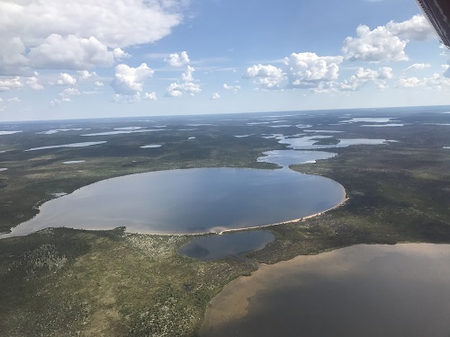
Figure 4. Aerial view of surface water in the study area (photo by Sarah Cooley).
Data Access
These data are available through the Oak Ridge National Laboratory (ORNL) Distributed Active Archive Center (DAAC).
ABoVE: AirSWOT Water Masks from Color-Infrared Imagery over Alaska and Canada, 2017
Contact for Data Center Access Information:
- E-mail: uso@daac.ornl.gov
- Telephone: +1 (865) 241-3952
References
Digital Globe. “EnhancedView Web Hosting Service.” 2018 (accessed July 2018). https://evwhs.digitalglobe.com/myDigitalGlobe/login
Fayne, J.V., L.C. Smith, L.H. Pitcher, and T.M. Pavelsky. 2019. ABoVE: AirSWOT Ka-band Radar over Surface Waters of Alaska and Canada, 2017. ORNL DAAC, Oak Ridge, Tennessee, USA. https://doi.org/10.3334/ORNLDAAC/1646
Kyzivat, E.D., L.C. Smith, L.H. Pitcher, J.V. Fayne, S.W. Cooley, M.G. Cooper, S. Topp, T. Langhorst, M. Harlan, C. Horvat, C. J. Gleason, and T.M. Pavelsky. A High-Resolution Airborne Color-Infrared Camera Water Mask for the NASA ABoVE Campaign. Remote Sensing, 2019, 11(18), 2163. https://doi.org/10.3390/rs11182163
Kyzivat, E.D., L.C. Smith, L.H. Pitcher, J. Arvesen, T.M. Pavelsky, S.W. Cooley, and S. Topp. 2018. ABoVE: AirSWOT Color-Infrared Imagery Over Alaska and Canada, 2017. ORNL DAAC, Oak Ridge, Tennessee, USA. https://doi.org/10.3334/ORNLDAAC/1643
McFeeters, S.K. The use of the Normalized Difference Water Index (NDWI) in the delineation of open water features. Int. J. Remote Sens. 1996, 17, 1425–1432. https://doi.org/10.1080/01431169608948714
Messager, M.L., B. Lehner, G. Grill, I. Nedeva, and O. Schmitt. 2016. Estimating the volume and age of water stored in global lakes using a geo-statistical approach. Nature Communications: 13603. https://doi.org/10.1038/ncomms13603. Data is available at www.hydrosheds.org.