Documentation Revision Date: 2019-03-29
Dataset Version: 1
Summary
The core of NASA AirSWOT is the Ka-band SWOT Phenomenology Airborne Radar (KaSPAR). Ka-band radar uses interferometry to measure surface elevation, particularly focusing on open surface water, producing novel swath water surface elevation measurements. AirSWOT collects two swaths of across-track interferometry data - between nadir and 1 km and between 1 km and 5 km, respectively - which can be used to obtain centimeter-level topographic maps of water surfaces. Only the outer-swath products are included in this release.
There are 1,547 radar output product files in GeoTIFF format provided with this dataset. This includes 768 files (128 swaths x 6 products) in original output at 3.6-m2 resolution in UTM coordinates, and 779 files (one for each ABoVE tile) provided in the ABoVE projection and clipped to the ABoVE 5-m2 C grid. A shapefile (.shp) is provided for visualization of all radar swaths with an index to the ABoVE grid files. This dataset also includes the following companion files: a *.kmz of the shapefile with an index to the ABoVE grid files, and 779 *.kml files of elevation data corresponding to the elevation product for the ABoVE grids.
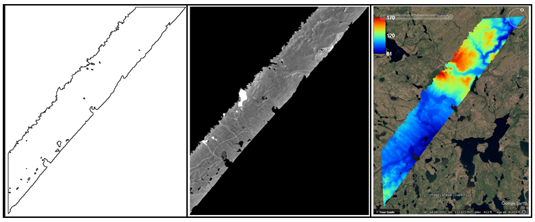
Figure 1. Example of AirSWOT radar products in ABoVE Projection at 3.6 m2 resolution, for a flight over the ABoVE C grid Ch065v034. Left: Shape for backscatter image. Middle: The magnitude image shows bright reflection in the near range, and no returns - yielding regions of no data in the far range. Right: Elevation product image.
Citation
Fayne, J.V., L.C. Smith, L.H. Pitcher, and T.M. Pavelsky. 2019. ABoVE: AirSWOT Ka-band Radar over Surface Waters of Alaska and Canada, 2017. ORNL DAAC, Oak Ridge, Tennessee, USA. https://doi.org/10.3334/ORNLDAAC/1646
Table of Contents
- Dataset Overview
- Data Characteristics
- Application and Derivation
- Quality Assessment
- Data Acquisition, Materials, and Methods
- Data Access
- References
Dataset Overview
AirSWOT is an airborne calibration and validation instrument for the upcoming Surface Water Topography Mission (SWOT) satellite. AirSWOT is capable of producing high resolution digital elevation models over land and water bodies. This dataset provides AirSWOT (https://swot.jpl.nasa.gov/airswot.htm) Ka-band (35.75 GHz) radar data products collected from an airborne platform over parts of Alaska and Canada during the period 2017-07-09 to 2017-08-17. Flights targeted specific surface water features, including rivers, lakes, ponds, and wetlands in the ABoVE domain. The radar data include six products: elevation (above the WGS84 ellipsoid), incidence angle, magnitude (backscatter), interferometric correlation (coherence), DHDPHI (incidence angle dependent height sensitivity), and error (estimated height random error, 1-sigma standard deviation). The flight lines were selected to span a full spectrum of permafrost conditions (permafrost-free to continuous permafrost, low to high ground ice content), ecosystems, climatic regions, topographic relief, and geological substrates across the ABoVE domain to investigate surface water responses to thawing permafrost and spatial and temporal variability in terrestrial water storage by measuring elevation and extent of surface waters. The data are provided in two forms: 1) the original output (outer-swath products only) at 3.6 m2 resolution in UTM coordinates from the AirSWOT processing group at the Jet Propulsion Laboratory (JPL), and 2) the ABoVE Projection at 3.6 m2 resolution, clipped to the ABoVE reference grid tiles using the C grid.
The core of NASA AirSWOT is the Ka-band SWOT Phenomenology Airborne Radar (KaSPAR). Ka-band radar uses interferometry to measure surface elevation, particularly focusing on open surface water, producing novel swath water surface elevation measurements. AirSWOT collects two swaths of across-track interferometry data - between nadir and 1 km and between 1 km and 5 km, respectively - which can be used to obtain centimeter-level topographic maps of water surfaces. Only the outer-swath products are included in this release.
Project: Arctic-Boreal Vulnerability Experiment
The Arctic-Boreal Vulnerability Experiment (ABoVE) is a NASA Terrestrial Ecology Program field campaign based in Alaska and western Canada between 2016 and 2021. Research for ABoVE links field-based, process-level studies with geospatial data products derived from airborne and satellite sensors, providing a foundation for improving the analysis and modeling capabilities needed to understand and predict ecosystem responses and societal implications.
Related Datasets:
Kyzivat, E.D., L.C. Smith, L.H. Pitcher, J. Arvesen, T.M. Pavelsky, S.W. Cooley, and S. Topp. 2018. ABoVE: AirSWOT Color-Infrared Imagery Over Alaska and Canada, 2017. ORNL DAAC, Oak Ridge, Tennessee, USA. https://doi.org/10.3334/ORNLDAAC/1643
Acknowledgments:
This research received funding from the NASA Terrestrial Ecology Program, grant number NNX17AC60A.
Special thanks go to The AirSWOT Processing Group at the Jet Propulsion Laboratory (JPL) who produced the original UTM products from the raw radar data. Members include Curtis Chen, Albert Chen, Michael Denbina, and Xiaoqing Wu.
Data Characteristics
Spatial Coverage: Alaska and Canada. In addition, this dataset includes an area in North Dakota, USA that was sampled as part of this campaign. It is not in the ABoVE Domain but may be displayed in the ABoVE Reference Grid.
ABoVE Reference Locations:
Domain: Core and Extended
State/territory: Alaska and Canada
ABoVE Grid: For files with data projected into the ABoVE grid, filenames have the respective ABoVE Grid C notation.
Spatial Resolution: The flight line data are recorded as thin swaths (< 5 km) along flight transects of varying length. The pixel size of original output is 3.6 m x 3.6 m. The resolution of data re-projected into the ABoVE C grid is also 3.6 m2.
Temporal Coverage: 2017-07-09 to 2017-08-17
Temporal Resolution: Variable, one to three collections per location
Study Area: (All latitude and longitude given in decimal degrees)
|
Site |
Westernmost Longitude |
Easternmost Longitude |
Northernmost Latitude |
Southernmost Latitude |
|---|---|---|---|---|
|
Alaska and Canada |
-149.847222 |
-98.626944 |
70.491388 |
46.847222 |
Data File Information
There are 1,547 radar output product files in GeoTIFF format provided with this dataset:
- 768 files (128 swaths x 6 products) in original output at 3.6-m2 resolution in UTM coordinates.
- 779 files, one for each of the represented ABoVE tiles in the ABoVE projection and clipped to the ABoVE 5-m2 C grid. These files contain all six products.
A shapefile (.shp) provides for visualization of the all radar swaths with an index to the ABoVE grid files.
Table 1. File names and descriptions
|
Data Files |
Descriptions and Naming Conventions |
|---|---|
| Radar Products in JPL UTM Projection | |
|
[product]_utm_[YYYYMMDDHHMMSS].tif
Example file name: magnitude_utm_20170817203741.tif |
768 GeoTIFFs (128 swaths x 6 products) in original output at 3.6-m2 resolution in UTM coordinates Radar products from JPL where [product] is one of these six types: correlation, height_sensitivity, error_bar, elevation, incidence_ angle, or magnitude. Products defined in Table 2 below. YYYYMMDDHHMMSS is the acquisition date (year, month, day, hour, minutes, seconds) |
|
Radar Products in the ABoVE C Grid Projection |
|
|
ABoVE.AirSWOT_Radar.[YYYYDDDHHMMSS].[ABoVE Grid C].001.[YYYYDDDHHMMSS].tif
Example file name: ABoVE.AirSWOT_Radar.2017189161653.Ch088v105.001.2018139101437.tif |
779 GeoTIFFs, one for each of the represented ABoVE tiles in the ABoVE projection and clipped to the ABoVE 5-m2 C grid. Radar products -- the six products described in Table 2 below -- are provided as 6-band GeoTIFFs. [YYYYDDDHHMMSS] is the acquisition date (year, day of year, hour, minutes, seconds), [ABoVE Grid C] is the ABoVE Grid C notation 001-version number [YYYYDDDHHMMSS] is the production date (year, day of year, hour, minutes, seconds) |
|
Shapefile |
|
|
AirSWOT_Radar_TileIndex.zip |
This shapefile (AirSWOT_Radar_TileIndex.shp) is provided in compressed format as a .zip file. The values are an index to the ABoVE C grid for a given location and may be used to identify the ABoVE projected GeoTIFF image(s) for that area. The file provides a smoothed outline of the swath data with areas of missing data (such as small lakes or ponds less than 1000 meters) removed. This file is also provided as a companion file in .kmz format for viewing in Google Earth. |
Radar products
Table 2. Description of the six radar data products included.
|
Radar data product |
Description |
Units/format |
Band (for ABoVE Projection GeoTIFF files) |
|---|---|---|---|
| elevation | Estimated height above the ellipsoid | Meters, referenced to WGS-84 | 1 |
|
incidence_ angle |
Incidence angle, estimated from reference DEM |
Radians |
2 |
|
magnitude
|
Backscatter-scaled square root of geometric mean of reference and secondary channel sigma0. |
Sigma0_in_db = 20*log10(.mag) |
3 |
|
correlation |
Interferometric correlation |
Dimensionless |
4 |
|
height_sensitivity |
Height sensitivity |
Meters/radian |
5 |
|
error_bar |
Estimated height error bar (1-sigma standard deviation) |
Meters |
6 |
Properties of the *.tif files:
JPL UTM projection
Bands: 1
No Data Value: -10000
Pixel size: 3.6 m x 3.6 m
EPSG: 32606 – 32614 (multiple UTM zones)
ABoVE projection
Bands: 6
No Data Value: -9999
Pixel size: 3.6 m x 3.6 m
EPSG: 102001 (ABoVE Projection -- Canada Albers Equal Area Conic)
Shapefile description:
File name: AirSWOT_Radar_TileIndex.shp
The only attribute is TileInd2. The values are an index to the ABoVE C grid for a given location and may be used to identify the ABoVE projected GeoTIFF image(s) for that area.
For example: TileInd2 = 2017225183621.Ch083v075.001
The outlines of the swath data in the shapefile have been smoothed -- areas of missing data (such as small lakes or ponds less than 1000 meters) were removed.
Companion files
There are 781 companion files provided with this dataset:
- The AirSWOT_Radar_TileIndex.shp data are provided in .KMZ format for quick reference to the ABoVE C grid tile and GeoTIFF files for a specific location.
- There are 779 KML files created for quick referencing in Google Earth for the elevation data only, in the ABoVE C grid. The files were created by spatially aggregating the re-projected and cropped elevation (.hgt) data by a factor of 10 which created 36-meter pixels. The files are provided in 779 directories as .zip files which include an image, elevation scale legend, and the .KML. These *.zip files correspond one-to-one with an elevation radar product.
- A .pdf of this guide document.
Application and Derivation
These data are designed to monitor spatial and temporal variability in terrestrial water storage by measuring elevation and extent of surface water. For more information on the application of these data, see: U.S.-Canada Collaboration to Build SWOT Calibration/Validation and Science Capacity for Northern Rivers and Wetlands. https://swot.jpl.nasa.gov/project-lsmith.htm
Quality Assessment
Uncertainty: Uncertainty is represented in the error data, which is the systematic error in the measurement reported as the estimate of the height error bar 1-sigma standard deviation.
Geolocation accuracy: This dataset was originally georeferenced to UTM coordinates from the radar SCH coordinate system. After reprojecting the data from UTM to the ABoVE specified format, the radar data still shows good agreement with other reference datasets such as Landsat data, Google Earth, as well as basemaps from ArcGIS and QGIS.
Missing data: Data at the near and far range are expected to have missing or noisy data, as the signal is low at the edges of the antenna footprint, and the signal from water is very weak at high incidence angles. This reduces the amount of signal that is returned to the sensor. In areas where the signal is weak, no data is produced for that area (pixel), resulting in a no data pixel value.
Unlike optical data, ground observations from radar data are not obscured by cloud cover. However, physical features such as the aircraft roll, layover or signal errors can contribute to missing data. Also, phase unwrapping errors may shift the geolocation of some ground features. This is rare and the data are quality controlled and corrected by the AirSWOT processing group at JPL prior to release (Fayne et al. in prep).
NOTE: In order to match the spatial reference of the coincident AirSWOT Camera data (available at Kyzivat, et al. 2018. https://doi.org/10.3334/ORNLDAAC/1643 ), as it uses manual tie points and registration, additional geoprocessing is ongoing to produce a version 2 dataset that aligns with the camera data.
Data Acquisition, Materials, and Methods
Study area
The data were collected using a NASA King Air B200 aircraft flying at ~8km altitude, over Alaska and Canada to conduct experimental remote sensing mapping of rivers, lakes and wetlands. In the ABoVE domain, data was acquired at many locations between July and August. Land heights are not expected to change between data collections, but water surface elevation is expected to change. Data were recorded over several areas including the Saskatchewan River, Saskatoon, Inuvik, Yukon River including Yukon Flats, Sagavanirktok River, Arctic Coastal Plain, Old Crow Flats, Peace-Athabasca Delta, Slave River, Athabasca River, Yellowknife, Great Slave Lake, Mackenzie River and Delta, Daring Lake, and others. More AirSWOT campaign information is available at https://swot.jpl.nasa.gov/airswot.htm.
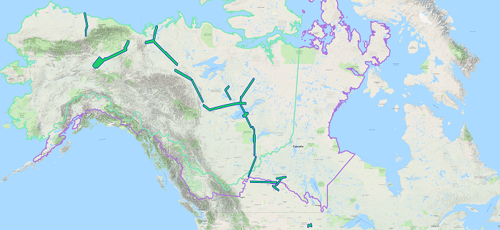
Figure 2. The ABoVE Domain with overlaid AirSWOT flights (Fayne et al. in prep).
Ka-band radar
NASA AirSWOT Ka-band Radar uses interferometry to measure surface elevation, particularly focusing on open surface water, producing novel swath water surface elevation measurements. The Ka-band (8.4 mm wavelength) interferometer was mounted on a NASA King Air B200 aircraft, collecting data at ~8km altitude.
The outer swath radar is left looking, with incidence angles ~4 - 27°, providing a nominal ~ 4 km swath width, with flight lines of varying lengths throughout the ABoVE domain (only outer-swath products are included in this release). The opposite headings provide data covering the full width of the swath of interest, as data over land in the near range or water in the far range may have weaker signal returns. This reduces the amount of signal that is returned to the sensor. At higher incidence angles, the signal over water often scatters away—particularly over very flat specular water bodies. This phenomenon is commonly called dark water because the water appears dark, or is not at all visible (as no data) in the radar images. (Fayne et al. in prep).
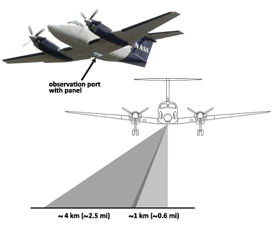
Figure 3. AirSWOT swath coverage.
Data Processing
This data contains the original output from the AirSWOT processing group at JPL, where the data are full-swath in UTM coordinates. The data are in GeoTIFF format and contain separate files for each radar product.
In addition, the data products were re-projected to the ABoVE Projection (Canada Albers Equal Area Conic, EPSG: 102001) and the data were clipped into the ABoVE tiles using the C grid (Loboda et al. 2017). The ABoVE-projection data are provided in GeoTIFF format with one file per tile and all six radar products in the same file.
In both UTM and ABoVE grid products, the elevations are referenced to a WGS84 ellipsoid, and the horizontal spatial resolution is ~3.6 meters.
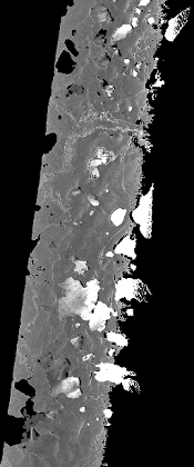
Figure 4. AirSWOT example swath. The image is acquired heading north and looking left (west). In the near range, the water is bright and in the far range the water is dark, seen as no data. Land is similarly dark in the near range (Fayne et al. in prep).
Keyhole Markup Language (.kml): KML files were created for quick referencing in Google Earth for the elevation data only. KML files were created by spatially aggregating the reprojected and cropped elevation (.hgt) data by a factor of 10, creating 36-meter pixels for the KML. The KML files use provided *.png files as the image data as well as the legend, and KML files to support the georeferencing of the *.png files.
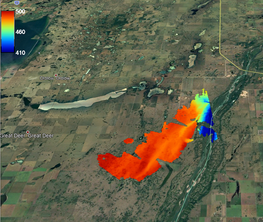
Figure 5. Example KML file shown in Google Earth with elevation legend (example from file ABoVE.AirSWOT_Radar.2017189163954.Ch088v106.001.2018139003155 )
Shapefile: Shapefile tiles of the swath data were created by: (1) creating a binary mask of the raster data, (2) converting the mask into a dissolved polygon, (3) buffering the polygon outwards 1000 m, and (4) buffering the polygon inwards 1000 m. This produces a smoothed outline of the swath data; areas of missing data (such as small lakes or ponds less than 1000 meters) were removed from the smoothed shape (Fayne et al. in prep).
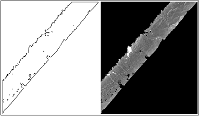
Figure 6. Left: Shape for backscatter image. Right: example backscatter image projected and clipped to ABOVE Grid –C (example from file ABoVE.AirSWOT_Radar_magnitude.2017221192908.Ch065v034.001.2018228010021.tif).
Data Access
These data are available through the Oak Ridge National Laboratory (ORNL) Distributed Active Archive Center (DAAC).
ABoVE: AirSWOT Ka-band Radar over Surface Waters of Alaska and Canada, 2017
Contact for Data Center Access Information:
- E-mail: uso@daac.ornl.gov
- Telephone: +1 (865) 241-3952
References
Fayne, J.V., L.C. Smith, L.H. Pitcher, and Y. Sheng. (In Prep). Mapping Surface Water with Ka-band Radar Water Likelihood (KARWL).
Loboda, T.V., E.E. Hoy, and M.L. Carroll. 2017. ABoVE: Study Domain and Standard Reference Grids, Version 2. ORNL DAAC, Oak Ridge, Tennessee, USA. https://doi.org/10.3334/ORNLDAAC/1527