Documentation Revision Date: 2016-04-29
Data Set Version: V1
Summary
The model was used in a spatially distributed mode (i.e., run cell-by-cell over a grid) over the four-state Northwest US region including Washington, Oregon, Montana, and Idaho. Landsat data were used to characterize disturbances, and Forest Inventory Analysis (FIA) plot data were used to parameterize the model.
There are 18 data files with this data set. This includes eight files in GeoTIFF (.tif) format in 25-m and 1000-m resolution, and 10 files in comma-separated (.csv) format.
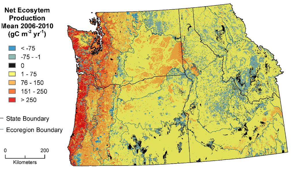
Figure 1. Mean net ecosystem production for 2006-2010 (from Turner et al., 2016).
Citation
Turner, D.P., W.D. Ritts, R.E. Kennedy, A.N. Gray, and Z. Yang. 2016. NACP Biome-BGC Modeled Ecosystem Carbon Balance, Pacific Northwest, USA, 1986-2010. ORNL DAAC, Oak Ridge, Tennessee, USA. http://dx.doi.org/10.3334/ORNLDAAC/1317
In addition to the data set citation, the following should also be referenced when using these data:
Turner, D.P., W.D. Ritts, R.E. Kennedy, A. Gray, and Z. Yang, 2016. Regional carbon cycle responses to 25 years of variation in climate and disturbance in the US Pacific Northwest. Reg Environ Change. doi: 10.1007/s10113-016-0956-9.Table of Contents
- Data Set Overview
- Data Characteristics
- Application and Derivation
- Quality Assessment
- Data Acquisition, Materials, and Methods
- Data Access
- References
Data Set Overview
Project: North American Carbon Program (NACP)
This data set provides Biome-BGC modeled estimates of carbon stocks and fluxes in the U.S. Pacific Northwest for the years 1986-2010. Fluxes include net ecosystem production (NEP), and net aboveground wood growth. Stocks include aboveground wood mass. Also present are mapped distributions of associated forest disturbances, distinguished by disturbance type (harvest, fire, pest/pathogen). The data are presented in a mapped form as well as in tabular summaries broken out by ownership and ecoregion. Maps of annual precipitation and temperature data are included for the years 1980-2010.
The model was used in a spatially distributed mode (i.e., run cell-by-cell over a grid) over the four-state Northwest US region including Washington, Oregon, Montana, and Idaho. Landsat data were used to characterize disturbances, and Forest Inventory Analysis (FIA) plot data were used to parameterize the model.
The North American Carbon Program (NACP) is a multidisciplinary research program designed to improve scientific understanding of North America's carbon sources and sinks and of changes in carbon stocks needed to meet societal concerns and to provide tools for decision makers.
Data Characteristics
Spatial Coverage: Pacific Northwest Region, USA
Spatial Resolution: GeoTIFFs are provided at 25 m and 1000 m resolution.
Temporal Coverage: Carbon data are for the years 1986 - 2010. Temperature and precipitation data are for the years 1980 - 2010.
Temporal Resolution: Annual.
Study Area (All latitudes and longitudes are given in decimal degrees.)
|
Site |
Westernmost Longitude |
Easternmost Longitude |
Northernmost Latitude |
Southernmost Latitude |
|
Pacific Northwest Region, USA (parts of Washington, Oregon, Montana, and Idaho) |
-127.2886.90 |
-109.678 |
50.88111 |
39.79639 |
Data File Information
NOTE: The data files provided by the author were used to produce the figures in Turner et al. (2016) . The files are named according to the figures in that paper. Files named "SFig_" correspond to the supplementary figures or charts for that paper.
GeoTIFFs
There are eight GeoTIFF files (*.tif) described below. There are common spatial properties to all files, and individual properties which are listed with each individual file description.
Spatial Data Properties (all files)
Parameters
Spatial Representation Type: Raster
Number of Bands: 1
Raster Format: GeoTIFF
units=m
Min_x= -2305000, Max_X= -1120000
Min_y= 2200000, Max_y= 3185000
Coordinates in decimal degrees:
|
West |
East |
North |
South |
|
-127.288 |
-109.678 |
50.88111 |
39.79639 |
Projection: North_America_Albers_Equal_Area_conic
False_Easting: 0.0
False_Northing: 0.0
Central_Meridian: -96.0
Standard_Parallel_1: 29.5
Standard_Parallel_2: 45.5
Latitude_Of_Origin: 23.0
Linear_Unit: Meter (1.0)
Geographic Coordinate System: GCS_North_American_1983
Angular_Unit: Degree (0.0174532925199433)
Prime_Meridian: Greenwich (0.0)
Datum: D_North_American_1983
Spheroid: GRS_1980
Semimajor Axis: 6378137.0
Semiminor Axis: 6356752.314140356
Inverse Flattening: 298.257222101
File descriptions
1) SFig1_pnw_epa_level3_ecoregions.tif: A modified version of the EPA Level 3 Ecoregions (Omernick 1987).
Spatial properties
Spatial resolution: 1,000 m
Number of columns: 1,185
Number of rows: 985
Fill value: 0
Data type: byte
Ecoregions in the GeoTIFF:
|
Class |
Short_description |
description |
|
0 |
nd |
nodata |
|
1 |
CR |
Coast Range |
|
2 |
PL |
Puget Lowlands |
|
3 |
WV |
Willamette Valley |
|
4 |
WC |
West Cascades |
|
9 |
EC |
East Cascades |
|
10 |
CP |
Columbia Plateau |
|
11 |
BM |
Blue Mountains |
|
12 |
SR |
Snake River Plain |
|
13 |
CB |
Central Basin and Range |
|
15 |
NR |
Northern Rockies |
|
16 |
IB |
Idaho Batholith |
|
17 |
MR |
Middle Rockies |
|
18 |
WB |
Wyoming Basin |
|
41 |
CA |
Canadian Rockies |
|
77 |
NC |
North Cascades |
|
78 |
KM |
Klamath Mountains |
|
80 |
NB |
Northern Basin and Range |
2) Fig2_pnw_LTMTBS_last_disturbance_type.tif: The most recent disturbance type. Disturbance types were extracted from the Monitoring Trends in Burn Severity (MTBS 2015) and Landtrendr (Kennedy et al., 2010) disturbance data sets.
Spatial properties
Spatial resolution: 1,000 m
Number of columns: 1,185
Number of rows: 985
Data type: float 32
Recent disturbance types in the GeoTIFF:
|
Class Name |
Description |
|
-1: No Disturbance |
Duration = 0, Magnitude = 0 |
|
1: Low Magnitude Fire |
MTBS override |
|
2: Moderate Magnitude Fire |
MTBS override |
|
3: High Magnitude Fire |
MTBS override |
|
4: Low Magnitude Cut |
1 <= LT Duration <= 4, 11 <= LT Magnitude <= 40 |
|
5: Moderate Magnitude Cut |
1 <= LT Duration <= 4, 41 <= LT Magnitude <= 70 |
|
6: High Magnitude Cut |
1 <= LT Duration <= 4, 71 <= LT Magnitude <= 100 |
|
7: Short Low Magnitude Pathogen |
5 <= LT Duration <= 12, 11 <= LT Magnitude <= 50 |
|
8: Short High Magnitude Pathogen |
5 <= LT Duration <= 12, 50 <= LT Magnitude <= 100 |
|
9: Medium Low Magnitude Pathogen |
13 <= LT Duration <= 20, 11 <= LT Magnitude <= 50 |
|
10: Medium High Magnitude Pathogen |
13 <= LT Duration <= 20, 51 <= LT Magnitude <= 100 |
|
11: Long Low Magnitude Pathogen |
21 <= LT Duration <= 28, 11 <= LT Magnitude <= 50 |
|
12: Long High Magnitude Pathogen |
21 <= LT Duration <= 28, 51 <= LT Magnitude <= 100
|
3) Fig3_pnw_mean_NEP_2006_2010.tif: Mean Annual NEP from 2006-2010 (kgC/m2/yr) derived by the PNWC Biome-BGC process model.
Spatial properties
Spatial resolution: 1,000 m
Number of columns: 1,185
Number of rows: 985
Data type: float 32
4) Fig1_pnw_nlcd2011_landcover.tif: A modified version of the 2011 National Land Cover Dataset (NLCD). These classes were reclassified.
Spatial properties
Spatial resolution: 25 m
Number of columns: 47,400
Number of rows: 39,400
Fill value: -128
Data type: byte
Band-Landcover class
|
Class |
Description |
|
2 |
Not Vegetated |
|
4 |
Cropland |
|
5 |
Grassland |
|
6 |
Shrubland |
|
7 |
Juniper Woodland |
|
8 |
Conifer Forest |
|
9 |
Deciduous Forest |
Reclassified Landcover classes
|
NLCD Code |
PNWC Code |
|
0 – Nodata |
0 No data |
|
11 - Open Water |
2 Not Vegetated |
|
12 - Perennial Ice/Snow |
2 Not Vegetated |
|
21 - Developed Open Space |
5 Grass |
|
22 - Developed Low Intensity |
2 Not Vegetated |
|
23 - Developed Medium Intensity |
2 Not Vegetated |
5) SFig3_pnw_standage_class.tif: A modified version of the GNN Standage age (http://lemma.forestry.oregonstate.edu/data). The GNN data set was available for Washington and Oregon. Robert Kennedy created a GNNtype standage for Idaho and Western Montana. We also used the MTBS-Landtrend disturbance layer as the basis for the youngest age class.
Spatial properties
Spatial resolution: 25 m
Number of columns: 47,400
Number of rows: 39,400
Fill value: 255
Stand Age Classes in the GeoTIFF:
|
Class |
Description |
|
0 |
Standage = 0 |
|
45 |
0 < Standage <= 60 |
|
80 |
60 < Standage <= 100 |
|
150 |
100 < Standage <= 200 |
|
250 |
Standage > 200 |
6) SFig2_pnw_ownership.tif: Public/Private ownership data.
Spatial properties
Spatial resolution: 25 m
Number of columns: 47,400
Number of rows: 39,400
Fill value: -1
Data type: byte
7) SFig4_pnw_total_annual_precip_1986_2010.tif: Mean annual precipitation from 1986 to 2010 derived from Daymet daily meteorological data (Thornton et al, 2014).
Spatial properties
Spatial resolution: 1,000 m
Number of columns: 1,185
Number of rows: 985
Data type: float 32
8) SFig4_pnw_mean_annual_temperature_1986_2010.tif: Mean annual temperature for 1986-2010 in degrees C derived from Daymet daily meteorological data (Thornton et al, 2014).
Spatial properties
Spatial resolution: 1,000 m
Number of columns: 1,185
Number of rows: 985
Data type: float 32
Comma separated (.csv) files
There are 10 comma-separated (.csv) data files with this data set. The ecoregions and four states of the PNW in the column headers are referenced by abbreviations provided in the table below.
Table 1. Pacific Northwest and Ecoregions
|
Ecoregion |
|
Pacific Northwest (PNW) |
|
Coast Range (CR) |
|
Puget Lowland (PL) |
|
Willamette Valley (WV) |
|
Klamath Mountains (KM) |
|
North Cascades (NC) |
|
West Cascades (WC) |
|
East Cascades (EC) |
|
Blue Mountains (BM) |
|
Northern Rockies (NR) |
|
Idaho Batholith (IB) |
|
Canadian Rockies (CA) |
|
Middle Rockies (MR) |
|
Oregon (OR) |
|
Western Montana (MT) |
|
Washington (WA) |
Data file descriptions
1) Table1_Ecoregion_mean_pct_disturbance.csv: Mean percent of forested areas disturbed; provided for the ecoregions CR,PL, WV, KM, NC, WC, EC, BM, NR, IP, CA, and MR by disturbances Harvest, Fire, and Pests/Pathogen.
| Column name | Units/format | Description |
|---|---|---|
| Ecoregion | text | Ecoregions where XX= CR,PL, WV, KM, NC, WC, EC, BM, NR, IP, CA, and MR |
| Harvest | percent | Percent of area disturbed from harvesting |
| Fire | percent | Percent of area disturbed from fires |
| Pest/Pathogen | percent | Percent of area disturbed from pests or pathogens |
2) Fig4_ Mean_NEP_ecoregion.csv: Mean NEP (g C/m2/yr) for the years 1986-2010, by ecoregion for each year.
|
Column name
|
Units |
Description
|
|
Year |
yyyy |
Year of data-1986-2010 |
|
XX_nep |
g C/m2/yr |
Mean NEP for each ecoregion for each year, 1986-2010, where XX = CR, PL, EC, WV, KM, WC, BM, NR, IB, CA, and MR.
|
3) Fig5_NEP_total_carbon_public_private.csv: Net ecosystem production (NEP), fire emissions, harvest removals, and net ecosystem carbon balance (NECB) for private forested land and public forested land, provided in Tg C/yr.
| Column name | Units/format | Description |
|---|---|---|
| C_source | text | Sources of carbon= NEP, Harvest, Fire emissions, or NECB |
| PNW_C_totals | TgC/yr | Carbon totals for the PNW area |
| PNW_C_Private | Tg C/yr | Carbon totals for privately owned forested land |
| PNW_C_Public | Tg C/yr | Carbon totals for public forested land |
4) SFig5_OR_CR_EC_abg_woodmass_FIA_BGC_agebin.csv: Aboveground wood biomass means for the Oregon Coast Range (OR-CR) and Oregon East Cascades (OR-EC) for observed FIA plot data and simulated (optimized Biome-BGC) biomass.
Values not reported, not applicable, or missing are provided as -9999.
| Column name | Units/format | Description |
|---|---|---|
| ageclass | numeric | Biomass age class (10 yr increments) from 20-160---20,30,40,etc. |
| OR-CR_FIA_stemmass | kgC/m2 | Aboveground wood biomass for the OR-CR ecoregion from FIA data |
| OR-CR_BGC_stemmass | kgC/m2 | Aboveground wood biomass for the OR-CR ecoregion from the Biome-BGC model |
| OR-EC_FIA_stemmass | kgC/m2 | Aboveground wood biomass for the OR-EC ecoregion from FIA data |
| OR-EC_BGC_stemmass | kgC/m2 | Aboveground wood biomass for the OR-EC ecoregion from the Biome-BGC model |
5) SFfig6_ prcp_tavg_1980_2010.csv: Mean annual temperature and annual precipitation over the Northwest region for years 1980-2010.
| Column name | Units/format | Description |
|---|---|---|
| Year | yyyy | Year of data (1980-2010) |
| prcp | cm | Precipitation in cm |
| t | degrees C | Mean annual temperature in degrees C |
6) SFig7_harvested_area_private_public.csv: Area of private and public forested land harvested for the years 1986-2010.
| Column name | Units/format | Description |
|---|---|---|
| Year | yyyy | Year of data (1986-2010) |
| PNW_private_hvst | km2 | Total PNW private forested area harvested |
| PNW_public_hvst | km2 | Total PNW public forested area harvested |
7) SFig8_harvested_area_intensity_class.csv: Area harvested by intensity class (1986-2010) over the study domain for the years 1986-2010.
| Column name | Unite/format | Description |
|---|---|---|
| Year | yyyy | Year of data (1986-2010) |
| Private_lowcut | km2 | Private land- low intensity harvested area |
| Private_modcut | km2 | Private land-moderate intensity harvested area |
| Private_highcut | km2 | Private land- high intensity harvested area |
| Public_lowcut | km2 | Public land- low intensity harvested area |
| Public_modcut | km2 | Public land- moderate intensity harvested area |
| Public_highcut | km2 | Public land- high intensity harvested area |
8) SFig9_burned_area_public_private.csv: Total burned area of private and public forested land for each year, 1986-2010.
| Column name | Units/format | Description |
|---|---|---|
| Year | yyyy | Year of data (1986-2010) |
| Private_burned_area | km2 | Total PNW private burned forested area |
| Public_burned_area | km2 | Total PNW public burned forested area |
9) SFig10_abg_woodmass_FIA_BGC.csv: Ecoregion mean aboveground wood mass (reported as kg C/m2) for Biome-BGC simulations and FIA plot data.
| Column name | Units/format | Description |
|---|---|---|
| Ecoregion | text | Data for the following ecoregions: CR, PL, WV, KM, NC, WC, EC, BM, NR, IB, CA, and MR |
| BGC_woodmass_mean | kg C/m2 | Mean aboveground wood mass produced from the BIOME-BGC simulation |
| FIA_woodmass_mean | kg C/m2 | Mean aboveground wood mass from FIA plot data |
10) SFig11_CFlux_ecoregion_ private_public.csv: Mean C (aboveground wood mass and net aboveground wood growth) by the carbon source (NEP), fires, harvesting, (NECB) and by ecoregions totals, ecoregions public and private lands (three columns for each ecoregion- total, public, and private).
Note: Ecoregions XX = PNW, CR, PL, EC, WV, KM, WC, BM, NR, IB, CA, MR, OR, WA, and MT.
| Column name | Carbon source |
| XX_Total_C_private_public | Total carbon from private and public forested land by source: NEP, Harvesting, Fire Emissions, and NECB |
| XX_Total_C_private | Total carbon from private forested land by source: NEP, Harvesting, Fire Emissions, and NECB |
| XX_Total_C_public | Total carbon from public forested land by source: NEP, Harvesting, Fire Emissions, and NECB |
Sample data entries from SFig11_CFlux_ecoregion_ private_public.csv:
|
Carbon_source |
PNW_total_C_private_public |
PNW_Total_C_private |
PNW_Total_C_public |
CR_Total_C |
CR_C_public |
CR_C_private |
|
NEP |
43.56579 |
58.52343 |
32.22572 |
202.7228 |
234.0523 |
180.3652 |
|
Harvest |
19.24919 |
37.43446 |
5.464104 |
103.3653 |
44.9123 |
145.0789 |
|
Fire Emission |
3.204932 |
0.480929 |
5.267691 |
0.07252 |
0.150493 |
0.016876 |
|
NECB |
21.11167 |
20.60805 |
21.49393 |
99.28493 |
188.9895 |
35.26944 |
Application and Derivation
These data are of value to the modeling community to better understand the terrestrial carbon cycle. To evaluate the possibilities for increased carbon sequestration, there is wide interest in quantifying carbon fluxes at more local and regional scales (Lu et al. 2013). The ecoregions are distinct with respect to climate, soil, and vegetation (USGS 2015).
Quality Assessment
Uncertainty in the simulated carbon stocks and flux estimates arise from errors in the spatially distributed inputs to the model, as well as from Biome-BGC model structure and parameter uncertainty. Uncertainties have previously been investigated in the distributed meteorological data (e.g., Hasenauer et al., 2003; Oyler et al., 2015), soil depth and texture (Peterman et al., 2014), disturbance mapping (Cohen et al., 2010), and stand age mapping (Ohmann and Gregory 2002). Observations of Biome-BGC parameters were compiled by White et al. (2000), and there is obvious species-level variation within a plant functional type. This issue was addressed by use of ecoregion-level parametrization based on (1) observations (e.g., foliar nitrogen concentration) and (2) parameter optimization (with reference to FIA observations) (Turner et al., 2016).
Efforts at validation of carbon stocks included comparison to aggregated FIA plot data. The comparison (SFig. 10) of ecoregion mean values suggests a positive bias in the simulated tree carbon stocks. The explanation may lie in a difference in the age class distributions in the wall-to-wall simulations versus the sample of FIA plots (Duane et al., 2010).
Data Acquisition, Materials, and Methods
Site description
The four-state (Oregon, Washington, Idaho, and Western Montana) Pacific Northwest regions (PNW) are distinct with respect to climate, soil, and vegetation (USGS 2015). Evergreen needleleaf forests dominate much of the region. The region is undergoing multiple changes in climate and vegetation relevant to the carbon cycle (Law and Waring 2015). A trend of climate warming over recent decades is observed in meteorological station data (e.g., Barnett et al. 2008; Pederson et al. 2010) albeit with controversy about the relative influence of internal climate variability versus anthropogenic factors (Abatzoglou et al. 2014; Johnstone and Mantua, 2014; Mote 2003) and possible artifacts in the observational record (Oyler et al. 2015). The forest disturbance regime in the northwest region is characterized by an increasing incidence of wildfire (Littell et al. 2009; Turner et al. 2015), generally attributed to climate warming. Pest and pathogen outbreaks are likewise increasing (Hicke et al. 2013), again associated with warming (Preisler et al. 2012). The drought in the Western USA from 2000 to 2004 strongly reduced the background carbon sink (Schwalm et al. 2012).
BIOME-BGC model simulation
A model run consisted of a spin-up, to bring slow turnover carbon pools (e.g. soil) into near equilibrium with the local climate, followed by one or two disturbance events (identified by year, type, magnitude, and duration). To limit the number of simulations required, only the 10 most frequent combinations of cover type and disturbance history in each 1-km2 grid cell were run. Area weighted mean values were then reported for carbon stocks and fluxes by year. Over 90% of the original study area was covered with this approach. The Biome-BGC model was applied in a spatially distributed mode (i.e., run cell-by-cell over a grid) over public and private land in the PNW.
Methods
The ecoregion boundaries are a modified version from Omernik (1987). To produce the file SFig1_pnw_epa_level3_ecoregions.tif, the data were resampled to 25 m and clipped to the PNW four state study region.
Ownership boundaries were from the Gap Analysis Program (GAP 2014). To produce the file SFig2_pnw_ownership.tif, the data were resampled to 25 m, clipped to the PNW four state study region, and reclassified.
The model was adapted to simulate disturbance and recovery associated with forest harvest (Law et al., 2004), wildfire (Meigs et al., 2011), and pests/pathogens (Turner et al., 2015). Mass balance was maintained by transfers among C pools and to the atmosphere at the time of a disturbance.
Landsat data were used to characterize disturbances, and Forest Inventory Analysis (FIA) data were used to parameterize the model. The 2010 land cover over a 25-m grid was from the National Land Cover Database (NLCD 2006) and was based on the Landsat data. To produce the file Fig1_pnw_nlcd2011_landcover.tif, the data were resampled to 25 m, clipped to the PNW four state study region, and reclassified.
Disturbance events
For the forest cover type, the disturbance history of each 25-m grid cell was specified based on Landsat observations. A time series (1985–2011) of Landsat images (one per year) were assembled over all forest areas and the trajectories and inflection points of a spectral vegetation index were evaluated for each 25-m pixel (Kennedy et al., 2010, 2012; Meigs et al., 2015). The disturbance type was classified as harvest, fire, or pest/pathogen. Abrupt disturbances (i.e., a sharp drop in the vegetation index) were classified as fire if they overlapped with the Monitoring Trends in Burn Severity data set (MTBS 2015), and otherwise as harvest. Non-abrupt disturbances were classified as pest/pathogen, and the remote sensing observations indicated a beginning year and a year of maximum impact.
To produce the file Fig2_pnw_LTMTBS_last_disturbance_type.tif, the following processing steps were followed:
- MTBS and Landtrendr data sets were resampled to 25 meters
- Clipped to the PNW study region
- Disturbance was called a fire if MTBS called it a fire
- Landtrendr was used to define the remaining disturbed pixels based upon the classification described above. Basically, short duration disturbances were assumed to be clear cuts. Longer duration disturbances were assumed to be pathogens.
Disturbances prior to 1985 were based on stand age, estimated from Landsat data using Gradient Nearest Neighbor (GNN) analysis (Ohmann and Gregory 2002). GNN-based stand age was not available for Idaho and Montana, so spectral relationships of Landsat data and stand age in eastern Oregon and Washington were used (with reference to the observed age class distributions from FIA data in Idaho and Montana) to estimate stand age in those states. The MTBS-Landtrendr disturbance layer was used to identify stands with age less than 30.
A class (bin) for disturbance magnitude and a class for duration were associated with each disturbance event (Turner et al., 2015), and for reporting purposes, the year of the event was assigned to the year of maximum magnitude.
To produce the file SFig3_pnw_standage_class.tif, the following processing steps were followed as described above:
- Data were resampled to 25 m,
- Clipped to the PNW study region,
- Lemma GNN Stand age for Washington and Oregon were combined with an in-house stand age layer for Idaho and Western Montana. The MTBS-Landtrendr disturbance layer was used to identify stands with age less than 30, and
- Stand age was reclassified.
Meteorological data
The 25-year time series of daily meteorological fields at 1-km resolution was from Daymet daily meteorological data for North America (Thornton et al, 2014). These data were developed by interpolation of meteorological station data using digital elevation maps and general meteorological principles (Thornton et al., 1997).
Data Access
This data is available through the Oak Ridge National Laboratory (ORNL) Distributed Active Archive Center (DAAC).
NACP Biome-BGC Modeled Ecosystem Carbon Balance, Pacific Northwest, USA, 1986-2010
Contact for Data Center Access Information:
- E-mail: uso@daac.ornl.gov
- Telephone: +1 (865) 241-3952
References
Abatzoglou, J.T., D.E. Rupp, and P.W. Mote (2014). Seasonal climate variability and change in the Pacific Northwest of the United States. J Clim 27:2125–2142. doi:10.1175/jcli-d-13-00218.1
Barnett, TP, Pierce DW, Hidalgo HG, Bonfils C, Santer BD, Das T, Bala G, Wood AW, Nozawa T, Mirin AA, Cayan DR, and Dettinger MD (2008). Human-induced changes in the hydrology of the western United States. Science 319:1080–1083. doi:10.1126/science.1152538
Cohen WB, Yang ZG, Kennedy R (2010) Detecting trends in forest disturbance and recovery 22 using yearly Landsat time series: 2. TimeSync - Tools for calibration and validation. 23 Remote Sens Environ 114:2911-2924. doi:10.1016/j.rse.2010.07.010
Duane MV, Cohen WB, Campbell JL, Hudiburg T, Weyermann D, Turner DP (2010). 36 Implications of two different field-sampling designs on landsat-based forest age maps 37 used to model carbon in Oregon forests. Forest Science 65:405-416.
GAP (2014). US Geological Survey, Gap Analysis Program (GAP). National Land Cover, Version 2. http://gapanalysis.usgs.gov/gaplandcover/data/. Accessed 10 Aug 2015.
Hasenauer, H., K. Merganicova, R. Petritsch, S.A. Pietsch, and P.E. Thornton (2003). Validating daily 12 climate interpolations over complex terrain in Austria. Agr Forest Meteorol 119:87-107.
Hicke, JA, Meddens AJH, Allen CD, Kolden CA (2013). Carbon stocks of trees killed by bark beetles and wildfire in the western United States. Environ Res Lett 8:8. doi:10.1088/1748-9326/8/3/035032
Johnstone, JA, Mantua NJ (2014). Atmospheric controls on northeast Pacific temperature variability and change, 1900–2012. Proc Natl Acad Sci USA 111:14360–14365. doi:10.1073/pnas.1318371111
Kennedy, RE, Yang ZG, Cohen WB (2010). Detecting trends in forest disturbance and recovery using yearly Landsat time series: 1. LandTrendr—temporal segmentation algorithms. Remote SensEnviron 114:2897–2910. doi:10.1016/j.rse.2010.07.008
Kennedy, RE, Yang ZQ, Cohen WB, Pfaff E, Braaten J, Nelson P (2012). Spatial and temporal patterns of forest disturbance and regrowth within the area of the Northwest Forest Plan. Remote Sens Environ 122:117–133. doi:10.1016/j.rse.2011.09.024
Law, BE, Turner D, Campbell J, Van Tuyl S, Ritts WD, and Cohen WB (2004). Disturbance and climate effects on carbon stocks and fluxes across Western Oregon USA. Global Change Biol 10:1429–1444. doi:10.1111/j.1365-2486.2004.00822.x
Law, B.E., and R.H. Waring (2015). Carbon implications of current and future effects of drought, fire and management on Pacific Northwest forests. For Ecol Manag 355:4–14. doi:10.1016/j.foreco.2014.11.023
Littell, JS, McKenzie D, Peterson DL, and Westerling AL (2009). Climate and wildfire area burned in western U.S. ecoprovinces, 1916–2003. Ecol Appl 19:1003–1021. doi:10.1890/07-1183.1
Lu, X.L. et al (2013). A contemporary carbon balance for the Northeast Region of the United States. Environ Sci Technol 47:13230–13238. doi:10.1021/es403097z.
Meigs, GW, Turner DP, Ritts WD, Yang ZQ, and Law BE (2011). Landscape-scale simulation of heterogeneous fire effects on pyrogenic carbon emissions, tree mortality, and net ecosystem production. Ecosystems 14:758–775. doi:10.1007/s10021-011-9444-8
Meigs GW, Kennedy RE, Gray AN, Gregory MJ (2015) Spatiotemporal dynamics of recent mountain pine beetle and western spruce budworm outbreaks across the Pacific Northwest region, USA. Remote Sens Environ 339:71–86. doi:10.1016/j.foreco. 2014.11.030
Mote, P.W. (2003). Trends in temperature and precipitation in the Pacific Northwest during the twentieth century. Northwest Sci 77:271–282.
MTBS (2015). Monitoring Trends in Burn Severity. http://www.mtbs.gov/. Accessed 10 Aug 2015
NLCD (2006). National land cover data. http://www.epa.gov/mrlc/nlcd.html. Accessed 10 Aug 2015
Ohmann JL, and Gregory MJ (2002). Predictive mapping of forest composition and structure with direct gradient analysis and nearest-neighbor imputation in coastal Oregon, U.S.A. Can J For Res 32:725–741. doi:10.1139/x02-011
Omernik, J.M. (1987). Ecoregions of the conterminous United States. Map (scale 1:7,500,000). Ann Assoc Am Geogr 77:118–125. doi:http://www.epa.gov/wed/pages/ecoregions/ecoregions.htm.Accessed 10 Aug 2015
Oyler, JW, Dobrowski SZ, Ballantyne AP, Klene AE, and Running SW (2015). Artificial amplification of warming trends across the mountains of the western United States. Geophys Res Lett 42:153–161. doi:10.1002/2014gl062803
Pederson, GT, Graumlich LJ, Fagre DB, Kipfer T, and Muhlfeld CC (2010). A century of climate and ecosystem change in Western Montana: what do temperature trends portend? Clim Change 98:133–154.
Peterman W, Bachelet D, Ferschweiler K, and Sheehan T (2014). Soil depth affects simulated carbon and water in the MC2 dynamic global vegetation model. Ecol Model 294:84–93. doi:10.1016/j.ecolmodel.2014.09.025
Preisler, HK, Hicke JA, Ager AA, and Hayes JL (2012). Climate and weather influences on spatial temporal patterns of mountain pine beetle populations in Washington and Oregon. Ecology 93:2421–2434.
Schwalm, CR, Williams CA, Schaefer K, Baldocchi D, Black TA, Goldstein AH, Law BE, Oechel WC, Kyaw TPU, and Scott RL. (2012). Reduction in carbon uptake during turn of the century drought in western North America. Nat Geosci 5:551–556.doi:10.1038/ngeo1529
Thornton, P.E., S.W. Running, and M.A. White (1997). Generating surfaces of daily meteorological variables over large regions of complex terrain. J Hydrol 190:214–251. doi:10.1016/s0022-1694(96)03128-9
Thornton, P.E., M.M. Thornton, B.W. Mayer, N. Wilhelmi, Y. Wei, R. Devarakonda, and R.B. Cook. 2014. Daymet: Daily Surface Weather Data on a 1-km Grid for North America, Version 2. Data set. Available on-line [http://daac.ornl.gov] from Oak Ridge National Laboratory Distributed Active Archive Center, Oak Ridge, Tennessee, USA. Date accessed: 2015/08/01. Temporal range: 1986/01/01-2010Y/12/31. Spatial range: N=50.00, S=42.00, E=-109.00, W=-125.00. http://dx.doi.org/10.3334/ORNLDAAC/1219
Turner, D.P., W.D. Ritts, R.E. Kennedy, A.N. Gray, and Z. Yang (2015). Effects of harvest, fire, and pest/pathogen disturbances on the West Cascades ecoregion carbon balance. Carbon Balance Manag 10:12. doi:10.1186/s13021-015-0022-9
Turner, D.P., W.D. Ritts, R.E. Kennedy, A.N. Gray, and Z. Yang. 2016. Regional carbon cycle responses to 25 years of variation in climate and disturbance in the US Pacific Northwest. Reg Environ Change; DOI 10.1007/s10113-016-0956-9 .
USDA (2011) U.S. Agriculture and Forestry Greenhouse Gas Inventory: 1990–2008. Technical Bulletin No. 1930.
USGS (2015). Omernik Level 3 Ecoregions for the U.S. (including Alaska) for Use as a Reference Data Collection. https://www. sciencebase.gov/catalog/folder/55c77f7be4b08400b1fd82d4?offset=60&max=30
White, M.A., P.E. Thornton, S.W. Running, and R.R. Nemani (2000). Parameterization and sensitivity 17 analysis of the BIOME-BGC terrestrial ecosystem model: net primary production 18 controls. Earth Interact 4:1-85.