CARVE: Monthly Atmospheric CO2 Concentrations (2009-2013) and Modeled Fluxes, Alaska

This data set reports monthly averages of atmospheric CO2 concentration from satellite and airborne observations between 2009 and 2013 and simulated present and future monthly concentrations and land-atmosphere CO2 flux for periods between 1990 and 2200. Atmospheric CO2 concentration measurements were obtained from Carbon in Arctic Reservoirs Vulnerability Experiment (CARVE) and NOAA Arctic Coast Guard (ACG) flights, the Greenhouse Gases Observing Satellite (GOSAT), and NOAA/ESRL vertical profile measurements at Poker Flat, Alaska (PFA). Present and future monthly CO2 concentrations and fluxes were simulated using the GEOS-Chem global tracer model and the Community Land Model, Version 4.5, for multiple regional flux and permafrost thaw scenarios.

The data are reported in 19 files in comma separated value (9) and NetCDF (10) file formats.

Project: Carbon in Arctic Reservoir Vulnerability Experiment (CARVE)

This data set reports monthly averages of atmospheric CO2 concentration from satellite and airborne observations between 2009 and 2013 and simulated present and future monthly concentrations and flux for periods between 1990 and 2200. Atmospheric CO2 concentration measurements were obtained from Carbon in Arctic Reservoirs Vulnerability Experiment and NOAA Arctic Coast Guard flights, the Greenhouse Gases Observing Satellite, and NOAA/ESRL vertical profile measurements at Poker Flat, Alaska. Present and future monthly CO2 concentrations and fluxes were simulated using the GEOS-Chem global tracer model (Parazoo et al., 2013) and the Community Land Model, Version 4.5 (Oleson et al., 2013; Koven et al., 2013; Swenson et al., 2012) for multiple regional flux and permafrost thaw scenarios.

The Carbon in Arctic Reservoirs Vulnerability Experiment (CARVE) is collecting detailed measurements of important greenhouse gases on local to regional scales in the Alaskan Arctic and demonstrating new remote sensing and improved modeling capabilities to quantify Arctic carbon fluxes and carbon cycle-climate processes. Ultimately, CARVE will provide an integrated set of data that will provide unprecedented experimental insights into Arctic carbon cycling.

Related publication:

Parazoo, N.C., R. Commane, S. Wofsy, C. Koven, C. Sweeney, D. Lawrence, J. Lindaas, R. Y.-W. Chang, and C.E. Miller (2016). Detecting Regional Patterns of Changing CO2 Flux in Alaska, Proc. Natl. Acad. Sci. (XX): XXXX-XXXX.

Spatial Coverage: Observed CO2 averages represent concentrations over Alaska. Outputs from the GEOSChem and CLM4.5 models have global coverage.

Spatial Resolution: 2.5 degrees Longitude x 2.0 degrees Latitude

Temporal Coverage

Observed CO2: 20090101-20131231

Simulated CO2: 19900101-22000101

Temporal Resolution: Monthly

 

Study Area

Site	Westernmost Longitude	Easternmost Longitude	Northernmost Latitude	Southernmost Latitude
Alaska	-180	-129.3	71.4	50.9
Global	-180	180	90	-90

 

Data Description

This data set provides monthly averages from airborne and satellite CO2 observations over Alaska for the period 2009-2013 in 9 comma separated value (*.csv) files. Simulated CO2 concentration and flux for present and future climates from a series of global transport model experiments are provided in 10 files in NetCDF (.nc) file format.

 

CSV files

Atmospheric CO2 concentrations are aggregated by month and vertical bin for each source of observations (GOSAT, CARVE, ACG, PFA).

File names: {Data_source}_Monthly_{Atmosphere_bin/Region}.csv

Data_source = one of 4 sources of CO2 concentration observations: GOSAT, CARVE, ACG, or PFA

Atmosphere_bin/Region = mixing layer (ML) or free troposphere (FT) for airborne observations (CARVE, ACG, or PFA); ALASKA, ARCTIC, MIDLAT for GOSAT

Header information: Each CSV has five columns: YEAR, MONTH, CO2, STD, NUM

YEAR = observation year

MONTH = observation month 

CO2 = CO2 concentration in parts per million (ppm)

STD = standard deviation of averaged CO2 observations for given month

NUM = count of CO2 observations for given month

 

NetCDF files 

Present

These simulations use year-specific CLM4.5 flux and winds to best represent observed conditions and inter-annual variability (TRANSPORT; see Section 5).

File names and descriptions:

CLM-TRENDY_Monthly.nc

Monthly fluxes (kg C km-2 s-1) from 2009 to 2013 driven by year-specific meteorological observations from the CRU-NCEP analysis (Wei et al., 2014).

GEOSCHEM-CLM-TRENDY_Monthly.nc

GEOS-Chem CO2 concentrations (ppm) for present day flux simulations from TRANSPORT runs. See Table 2 for layer names and descriptions.

Table 2. Layer names and descriptions for GEOSCHEM-CLM-TRENDY_Monthly.nc

Layer	Description
gc-control	Global fluxes set to CLM-TRENDY
gc-alaska-off	Global fluxes set to CLM-TRENDY; Alaska fluxes set to zero
gc-arctic-off	Global fluxes set to CLM-TRENDY; Arctic fluxes set to zero

 

Future

These simulations use time-varying winds from 2000-2010 and 6 sets of decadal CLM4.5 fluxes for present day (hist, 1990-2010) and future scenarios (15yr, 2005-2015; 30yr, 2020-2030; 50yr, 2040-2050; 100yr, 2090-2100; 200yr, 2190-2200). They are further divided into simulations to test CO2 sensitivity to flux changes in Alaska (ALASKA-ON), the Arctic (ARCTIC-ON), and at global scale (GLOBAL-ON). Two permafrost thaw scenarios are simulated: (1) FUTURE-DEEP, assumes deep permafrost carbon is active; (2) FUTURE-SHALLOW, deep soil decomposition is disabled (see Section 5).

File names and descriptions:

CLM-FUTURE-DEEP_Monthly.nc & CLM-FUTURE-SHALLOW_Monthly.nc

Monthly fluxes (kg C km-2 s-1) for present and future scenarios forced by time-varying meteorology and constant pre-industrial CO2, for active (FUTURE-DEEP) and inactive (FUTURE-SHALLOW) scenarios for deep permafrost carbon. 

CLM-FUTURE-DEEP_CO2_Monthly.nc

Monthly fluxes (kg C km-2 s-1) for present and future scenarios driven by time-varying meteorology and time-varying CO2 with active deep permafrost carbon.

GEOSCHEM-CLM-DEEP_ALASKA-ON_Monthly.nc & GEOSCHEM-CLM-DEEP_ARCTIC-ON_Monthly.nc

GEOSCHEM CO2 concentrations (ppm) for ALASKA-ON and ARCTIC-ON flux simulations with active deep permafrost carbon.

GEOSCHEM-CLM-DEEP_GLOBAL-ON_Monthly.nc

GEOSCHEM CO2 concentrations (ppm) for GLOBAL-ON flux simulations with active deep permafrost carbon.

GEOSCHEM-CLM-SHALLOW_ALASKA-ON_Monthly.nc

GEOSCHEM CO2 concentrations (ppm) for ALASKA-ON flux simulations with inactive deep permafrost carbon.

GEOSCHEM-CLM-SHALLOW_ARCTIC-ON_Monthly.nc

GEOSCHEM CO2 concentrations (ppm) for ARCTIC-ON flux simulations with inactive deep permafrost carbon. 

Layer names: {Permafrost_scenario} _{CLM_simulation_period} _{Simulated_flux_region}

Where:

Permafrost_scenario = deep or shallow; indicates whether deep permafrost carbon was active in the simulation

CLM_simulation_period = indicates the simulation period as based on the parameters defined in Table 3.

Simulated_flux_region = Alaska, arctic, or global; indicates which region for which CO2 flux was active in the simulation run

Table 3. CLM simulation period layers

Layer name	CLM Simulation Period
*-hist-*	1990-2010
*-15yr-*	2005-2015
*-30yr-*	2020-2030
*-50yr-*	2040-2050
*-100yr-*	2090-2100
*-200yr-*	2190-2200

Atmospheric CO2 observations provide spatially and temporally integrated constraints of CO2 exchange on regional to pan-Arctic scales. In situ observations have been limited primarily to a small network of surface towers and infrequent, short duration airborne campaigns designed primarily to detect the pan-Arctic background CO2 signal. Comparison of monthly CO2 averages across airborne and satellite data sets in Alaska show high consistency of seasonal and inter-annual variability and long term growth. Each platform and underlying sampling strategy provides an important strength needed to characterize the Alaskan CO2 seasonal cycle. When aggregated over the growing season, GOSAT provides high spatial coverage throughout the Arctic-boreal zone. PFA captures the full annual cycle within the continental interior. CARVE and ACG capture spatial variability during the growing season, and CARVE provides high quantity measurements and captures high frequency time and space variations near the surface within the continental interior.

Simulated flux data assesses the detectability of Alaskan carbon cycle signals under present climate and future warming scenarios. CO2 flux simulations show changes in seasonal CO2 exchange with warming. Simulated CO2 concentrations show sensitivity of atmospheric CO2 seasonal cycle amplitude to change in Alaskan CO2 flux.

Observed CO2

CO2 observations are averaged by month and vertical bin and subject to significant variability driven by weather and spatial gradients. The variability is quantified as monthly standard deviations in the CO2 observations.

Simulated CO2

Changes in CO2 seasonal cycle amplitude are driven by slow changes in uptake and inter-annual variability in uptake and transport. Uncertainty in projected seasonal cycle amplitude change was quantified as the standard deviation of year-to-year variability across 10 years. 

Uncertainty analyses are further described in the related publication (Parazoo et al, 2016).

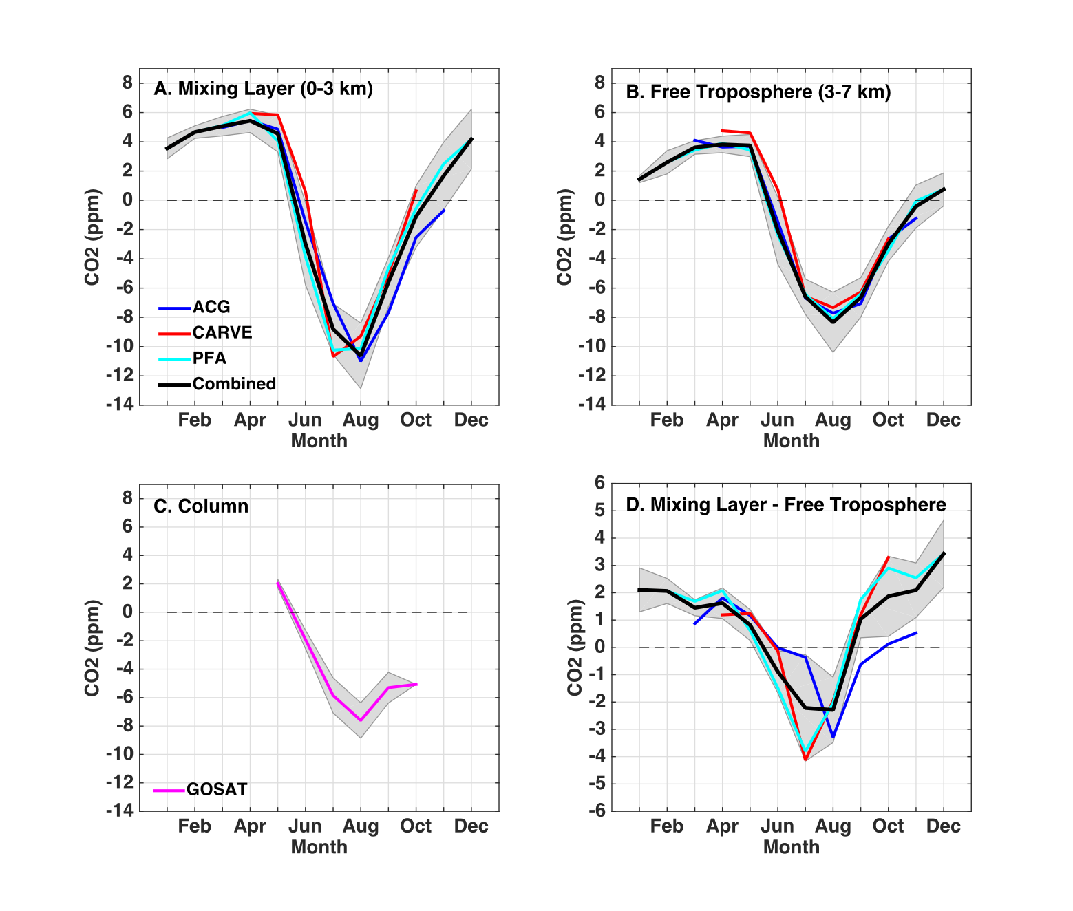
Figure 2. Observed CO2 seasonal cycles from satellite and airborne instruments (from Parazoo et al., 2016).

Observed CO2

• Greenhouse Gases Observing Satellite (GOSAT; Kuze et al., 2009) CO2 retrievals have produced full coverage of the growing season (April to September) and partial coverage of spring and fall shoulder seasons at Alaska to pan-Arctic scales since 2009. An average of 274 samples were obtained per year for the Alaskan domain (55-72°N, 170-140°W) and 4,000-5,000 per year for the pan-Arctic (55-72°N, 180°W-180°E).
• CARVE campaign flights over much of the Alaskan interior were conducted for a period of 2 weeks per month from May to September in 2012 and April to October in 2013 with 4 to 10 flights per campaign and 75 total tracks collected over the two years (Miller and Dinardo, 2012). CARVE surveys produced high-frequency in situ measurements of the lowest 500 m above the surface using a cavity ring-down spectroscopy instrument.
• Arctic Coast Guard (ACG) flights collected high-frequency in situ measurements of CO2 concentration across more than 50 flights with a cavity ring-down spectroscopy instrument. Round trip flights between Kodiak and Barrow, Alaska took place from early March to late November from 2009 to 2013. An average of 3 vertical profiles were measured per flight.
• Whole air samples at altitudes between 500 and 8,000 masl were collected during NOAA/ESRL flights over the Poker Flat Alaska Research Range (PFA) , northeast of Fairbanks, Alaska every 2 to 4 weeks beginning in 2000.

All aircraft data sets were filtered for biomass burning using onboard CO measurements and a high CO screen of 150 ppb, then separated into mixing layer (ML) and free troposphere (FT) bins. All available data in the lowest 3 km asl (<700 millibars) were averaged for the ML and from 3-7 km asl (700-500 millibars) for the FT. 

CO2 observations from each airborne campaign (GOSAT, CARVE, ACG, PFA) were averaged by month for the ML and FT bins and reported in separate CSV files. GOSAT observations were averaged by month for Alaska (55-72°N, 170-140°W), Arctic (55-90°N, 180°W-180°E), and mid-latitude (55°N-55°S, 180°W-180°E) regions and reported in separate CSV files.

Simulated CO2

Atmospheric CO2 concentrations were simulated using the GEOS-chem global tracer model (Parazoo et al., 2013) forced by assimilated meteorological fields and surface CO2 flux from land, ocean, and fossil fuel sources. Monthly CO2 output was sampled during midday (10-18 LST), averaged across all Alaskan land grid points (55-72°N, 170-140°W), and binned vertically into the ML and FT. Present and future land-atmosphere CO2 fluxes were simulated through experiments based on two configurations of the Community Land Model, Version 4.5 (CLM4.5; Oleson et al., 2013; Koven et al., 2013; Swenson et al., 2012). 

Present

The experiments running the first of the two configurations, denoted TRANSPORT, focused between 2009-2013 to examine sensitivity of observed CO2 seasonal cycles to Alaskan CO2 flux. These simulations use year-specific CLM4.5 flux and winds to best represent observed conditions and inter-annual variability. Three variants were considered: (1) CONTROL, a baseline run with all fluxes turned on; (2) ALASKA-OFF, an Arctic influence run with Alaskan fluxes set to zero (55-72°N, 170-140°W); (3) ARCTIC-OFF, the long-range transport run with Arctic fluxes set to zero (55-90°N, 180°W-180°E).

Future

The experiments running the second of the two configurations focused on the ability of current observing strategies to detect changes in CO2 flux patterns resulting from projected climate-induced changes in the Arctic-Boreal Zone carbon cycle. These simulations used time varying winds from 2000-2010 and 6 sets of decadal CLM4.5 fluxes for present day (hist, 1990-2010) and future (15yr, 2005-2015; 30yr, 2020-2030; 50yr, 2040-2050; 100yr, 2090-2100; 200yr, 2190-2200) scenarios. These were further divided into simulations to test CO2 sensitivity to flux changes in Alaska (ALASKA-ON), the Arctic (ARCTIC-ON), and at global scale (GLOBAL-ON). CLM4.5 was configured as described in two recent permafrost studies (Koven et al., 2015, Lawrence et al., 2015) and forced by time-varying meteorology corresponding to historical and future climates, with modeled photosynthesis driven by constant preindustrial CO2. The two scenarios for permafrost thaw are denoted FUTURE-DEEP and FUTURE-SHALLOW. FUTURE-DEEP assumes deep permafrost carbon is active. Deep soil decomposition is disabled in FUTURE-SHALLOW. These experiments decouple changing dynamics of surface soils from deep soils and isolate the potential contributions from permafrost layers.

Koven, C.D., et al. (2013). The effect of vertically-resolved soil biogeochemistry and alternate soil C and N models on C dynamics of CLM4. Biogeosciences 10(11): 7109-7131.

Koven, C.D., D.M. Lawrence, and W.J. Riley (2015). Permafrost carbon- climate feedback is sensitive to deep soil carbon decomposability but not deep soil nitrogen dynamics. P. Natl. Acad. Sci. 112(12): 3752-3757.

Kuze, A., H. Suto, M. Nakajima, and T. Hamazaki (2009). Thermal and near infrared sensor for carbon observation Fourier-transform spectrometer on the Greenhouse gases observing satellite for greenhouse gases monitoring. Appl. Optics 48: 6716-6733.

Lawrence, D.M., C.D. Koven, S.C. Swenson, W.J. Riley, and A.G. Slater (2015). Permafrost thaw and resulting soil moisture changes regulate projected high-latitude CO2 and CH4 emissions. Env. Res. Lett. 10: 094011.

Miller, C.E. and S. J. Dinardo, "CARVE: The Carbon in Arctic Reservoirs Vulnerability Experiment," Aerospace Conference, 2012 IEEE, Big Sky, MT, 2012, pp. 1-17. doi: 10.1109/AERO.2012.6187026

Oleson, K.W., et al. (2013). Technical Description of version 4.5 of the Community Land Model (CLM). NCAR Technical Note NCAR/TN-503+STR, DOI:10.5065/D6RR1W7M.

Parazoo, N.C., et al. (2013). Interpreting seasonal changes in the carbon balance of southern Amazonia using measurements of XCO2 and chlorophyll fluorescence from GOSAT, Geophys. Res. Lett. 40:1-5.

Parazoo, N.C., R. Commane, S. Wofsy, C. Koven, C. Sweeney, D. Lawrence, J. Lindaas, R. Y.-W. Chang, and C.E. Miller (2016). Detecting Regional Patterns of Changing CO2 Flux in Alaska, Proc. Natl. Acad. Sci. Online Early. doi:10.1073/pnas.1601085113

Swenson, S.C., D.M. Lawrence, and H. Lee (2012). Improved simulation of the terrestrial hydrological cycle in permafrost regions by the Community Land Model. J. Adv. Model Earth Sy. 4(3), DOI: 10.1029/2012MS000165.

Wei, Y., S. Liu, D. Huntzinger, A. Michalak, N. Viovy, W. Post, C. Schwalm, K. Schaefer, A. Jacobson, and C. Lu (2014). The North American Carbon Program Multi-scale Synthesis and Terrestrial Model Intercomparison Project-Part 2: Environmental driver data, Geoscientific Model Development 7: 2875-2893.