Get Data
Revision Date: July 7, 2015
Summary:
This data set provides estimates of aboveground biomass (AGB) for defined land cover types within World Wildlife Fund (WWF) ecoregions across the boreal biome of eastern and western Eurasia, roughly between 50 and 70 degrees N. The study focused on within-growing-season data, i.e. leaf-on conditions.
The AGB estimates were derived from a series of models that first related ground-based measured biomass to airborne data collected with an Optech Airborne Laser Terrain Mapper (ALTM) 3100, and a second set of models that related the airborne estimates of biomass to Geoscience Laser Altimeter System (GLAS) LiDAR canopy structure measurements. The ground, airborne, and GLAS measurements were used to formulate the models needed to generate biomass predictions for western Eurasia. Eastern Eurasia employed a two-phase approach relating field measurements directly to the GLAS measurements without the airborne intermediary. The GLAS LiDAR biomass estimates were extrapolated by land cover types and ecoregions across the entire biome area.
The study compiled remotely sensed forest structure data collected in June of 2005 and 2006 from the GLAS LiDAR instrument aboard the NASA Ice, Cloud, and land Elevation (ICESat) satellite and from an Optech Airborne Laser Terrain Mapper (ALTM) 3100 airborne instrument flown in Southeast Norway over both the ground plots and the ICESat GLAS flight path. For a consistent biome-level analysis, ecoregions contained within the boreal forest biome were identified by the World Wildlife Fund's (WWF) ecoregion map of the world (Olson et al., 2001). MODIS MOD12Q1 land cover products (2004) were used to identify land cover types for stratification purposes within eco-regions. The ground-based measurements are not provided with this data set.
There are seven data files with this data set which includes four files in comma-separated format (.csv) and three GeoTIFF files (.tif).
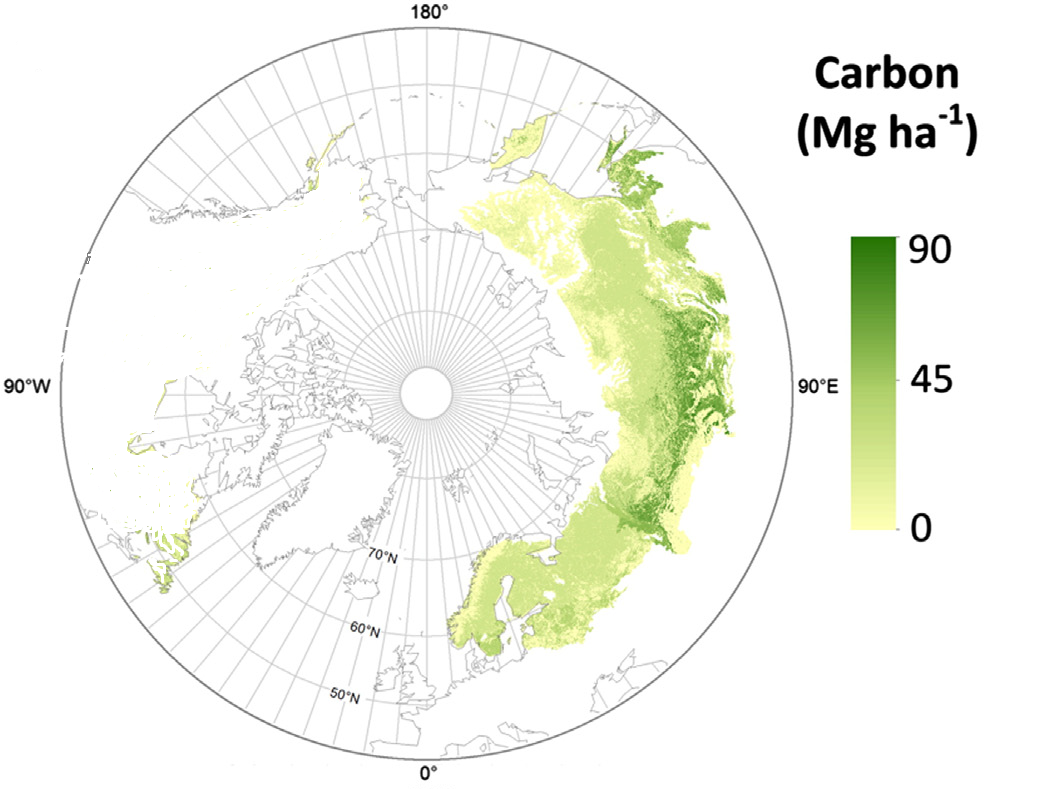
Figure 1. Eurasia boreal forests aboveground carbon estimates (Neigh et al., 2013).
Data Citation:
Cite this data set as follows:
Neigh, C.S., R.F. Nelson, K.J. Ranson, H. Margolis, P.M. Montesano, G. Sun, V. Kharuk, E. Naesset, M.A. Wulder, and H.E. Anderson. 2015. LiDAR-based Biomass Estimates, Boreal Forest Biome, Eurasia, 2005-2006. Data set. Available online [http://daac/ornl.gov/] from Oak Ridge National Laboratory Distributed Active Archive Center, Oak Ridge, Tennessee, USA. http://dx.doi.org/10.3334/ORNLDAAC/1278
Table of Contents:
- 1 Data Set Overview
- 2 Data Characteristics
- 3 Applications and Derivation
- 4 Quality Assessment
- 5 Acquisition Materials and Methods
- 6 Data Access
- 7 References
1. Data Set Overview:
This data set provides estimates of aboveground biomass (AGB) for defined land cover types within World Wildlife Fund (WWF) ecoregions across the boreal biome of eastern and western Eurasia, roughly between 50 and 70 degrees N. The study focused on within-growing-season data, i.e. leaf-on conditions.
The AGB estimates were derived from a series of models that first related ground-based measured biomass to airborne data collected with an Optech Airborne Laser Terrain Mapper (ALTM) 3100, and a second set of models that related the airborne estimates of biomass to Geoscience Laser Altimeter System (GLAS) LiDAR canopy structure measurements. The ground, airborne, and GLAS measurements were used to formulate the models needed to generate biomass predictions for western Eurasia. Eastern Eurasia employed a two-phase approach relating field measurements directly to the GLAS measurements without the airborne intermediary. The GLAS LiDAR biomass estimates were extrapolated by land cover types and ecoregions across the entire biome area.
The study compiled remotely sensed forest structure data collected in June of 2005 and 2006 from the GLAS LiDAR instrument aboard the NASA Ice, Cloud, and land Elevation (ICESat) satellite and from an Optech Airborne Laser Terrain Mapper (ALTM) 3100 airborne instrument flown in Southeast Norway over both the ground plots and the ICESat GLAS flight path. For a consistent biome-level analysis, ecoregions contained within the boreal forest biome were identified by the World Wildlife Fund's (WWF) ecoregion map of the world (Olson et al., 2001). MODIS MOD12Q1 land cover products (2004) were used to identify land cover types for stratification purposes within eco-regions. The ground-based measurements are not provided with this data set.
Related Data Set:
NACP LiDAR-based Biomass Estimates, Boreal Forest Biome, North America, 2005-2006
2. Data Characteristics:
Spatial Coverage
Boreal forest biome of Eurasia, roughly between 50 and 70 degrees N.
Spatial Resolution
1,172 m between sequential GLAS shots which are 60-m in diameter.
Temporal Resolution
One time estimates.
Temporal Coverage
The data cover the period 2005-06-08 to 2006-06-26.
Site boundaries: (All latitude and longitude given in decimal degrees, datum: WGS84)
| Site (Region) | Westernmost Longitude | Easternmost Longitude | Northernmost Latitude | Southernmost Latitude |
|---|---|---|---|---|
| Eurasia (boreal biome) | 68.166527 | 77.979637 | 66.329552 | 51.183777 |
Data File Information
There are seven data files with this data set which includes four comma-separated files (.csv) files and three GeoTIFF (.tif) files. The .csv files include AGB estimates generated from an IDL program as well as the model input variables from GLAS, and the ASTER DEM. The ground-based measurements are not provided with this data set. The three .tif files provide: (1) AGB in Mg/ha for all regions combined, (2) model-based standard error of AGB in Mg/ha, and (3) relative error of the AGB in Mg/ha for all three combined regions.
Biomass Data files (.txt format)
AGB data are provided for eastern and western Eurasia.
- The data pertain only to high-graded GLAS shots on slopes <= 20 degrees (avslope).
- Within the model, land cover not classified as wetlands, hardwood, conifer, mixedwood, or burn is equal to zero biomass.
- Total biomass = stems + branches + foliage and is reported in tons/ha.
The data files provide:
(1) AGB for individual ecozones, across flight lines (FL) and systematic samples, for wetlands, hardwood, conifer, mixed wood, and burned areas, as well as estimates from four systematic samples with the number of GLAS shots.
(2) AGB biomass stratum estimates by ecozone.
(3) AGB estimates across all strata (five) and ecozones.
Table 1. Data file names and general descriptions
Note: L3c, L3f, L2a, and L3a refer to the GLAS acquisition numbers (refer to Neigh et al., 2013 for additional information).
| FILE NAME | DESCRIPTION |
|---|---|
| EA_east_L3c_hg.csv | Data file for eastern Eurasia in .csv format. |
| EA_east_L3f_hg.csv | Data file for eastern Eurasia in .csv format |
| EA_west_L2a_hg.csv | Data file for western Eurasia in .csv format |
| EA_west_L3a_hg.csv | Data file for western Eurasia in .csv format |
Model Input Data Variables
Tables 2-3 identify the names, units, and descriptions for all the variables in the model input data files. Each table contains descriptions for the variables and their respective sources.
Table 2. GLAS Variables (GLA01 and GLA14 source). Additional information on GLAS variables can be found at the National Snow & Ice Data Center (Zwally et al., 2011; Zwally et al., 2014).
| Variable | Units/format | Description |
|---|---|---|
| rec_ndx | GLAS record index | |
| shotn | Shot number (1 through 40 shots when no pulses are missing) | |
| date | Days since January 1, 2003 | |
| lat | degrees | Latitude in decimal degrees |
| lngtd | degrees | Longitude in decimal degrees. Negative values for western hemisphere |
| elev | The elevation of the waveform centroid directly from GLA14. According to the GLAS documentation, this is the “surface elevation with respect to the ellipsoid at the spot location determined by range using the land-specific fitting procedure after all instrument corrections, atmospheric delays and tides have been applied”. | |
| elvdiff | The adjusted “elev” to geoid surface height. | |
| wfl0,lead,trail | m | Waveform height indices. The trailing edge extent (Fig. 2) is most closely related to terrain slope; the leading edge extent (Fig. 2) is related to canopy height variability and must be applied to estimate mean tree height rather than maximum tree height. The trailing edge extent is calculated from the waveform as the height difference between the lowest elevation at which the signal strength of the waveform is half of the maximum signal above the background noise value, and the elevation of the signal end. Similarly, the leading edge extent is determined as the height difference between the elevation of the signal start and the first elevation at which the waveform is half of the maximum signal above the background noise value. Refer to Lefsky et al., 2007 for more detailed explanation |
| MedH | m | Median canopy height |
| MeanH | m | Mean canopy height |
| QMCH | m | Quadratic mean canopy height (Lefsky 1999). If there was difficulty in separating the returns from the canopy and ground, these heights could not be calculated, and were therefore set to zero |
| Centroid, wflen, h14 | m | Waveform centroid (Centroid) and top canopy height (h14) relative to the first Gaussian peak. "wflen" is the distance from signal beginning to ending |
| ht1 | m | The distance from signal beginning to ground peak as calculated from the waveform. |
| ht2 | m | The ht1 distance with a correction for the widening of the ground peak due to slope. |
| ht3 | m | Height that is further corrected for off-nadir looking using beam_ coelev |
| ht4 | m | The height resulting from removing the half width of the laser pulse, so for a bare surface, ht4 should close to zero. |
| fslope | degrees | The angle between vertical and the line from signal beginning to the highest waveform peak. |
| eratio | The ratio of canopy to ground energy. | |
| Senergy | digital counts | The energy from ground. Note that the ratio of canopy energy to total energy is eratio/(1+eratio). |
| h10, h20, h25, h30, h40, h50, h60, h70, h75, h80, h90, h100 | m | Energy indices (relative to ground peak) for each respective percentile. |
| gdpamp | digital counts | Amplitude of the ground peak |
| mjp1loc, mjp2loc, mjp3loc, mjp4loc, mjp5loc, mjp6loc | m | Locations of the six major peaks |
| mjp1amp, mjp2amp, mjp3amp, mjp4amp, mjp5amp, mjp6amp | digital counts | Amplitude of locations of six major peaks |
| satndx | The count of the number of gates in a waveform which have an amplitude greater than or equal to i_satNdxTh (threshold). The value 126 means 126 or more gates are above the saturation index threshold (i_satNdxth). | |
| npk | number | Number of Gaussian peaks retrieved from the waveform. Officially, the number of peaks in the waveform produced by the Gaussian filtering, using alternate parameters. |
| gh1, gh2, gh3, gh4, gh5, gh6 | m | Height of each Gaussian solved for up to six using alternate parameters. The value 99999 signifies missing data if there are not 6 peaks. The algorithm looks for up to six Gaussian peaks in a waveform return but there are often not six peaks to be found. |
| gam1, gam2, gam3, gam4, gam5, gam6 | 0.01 volts | Amplitude of each Gaussian solved for (up to six), using the alternate parameters. Units = 0.01 volts. |
| gs1, gs2, gs3, gs4, gs5, gs6 | 0.001 ns | Width (sigma) of each Gaussian solved for (up to six), using alternate parameters. Units = 0.001 ns. |
| ga1, ga2, ga3, ga4, ga5, ga6 | 0.01 volts x ns | Area under each of the Gaussians solved for (up to six), using alternate parameters. Units = 0.01 volts x ns. |
Table 3. WWF Ecozone, ASTER and Other Variables for Eurasian Data: An IDL program was adapted to extract the WWF ecozone code, ASTER slope, and other variable for each GLAS pulse and attach it to the GLAS data file.
| Variable | Units/format | Description |
|---|---|---|
| Slope_aster | degrees | ASTER GDEM V1 (>500 tiles) were processed using ENVI topographic modeler, calculating min/max slope within a 90 x 90 m window. Elevations < 3 m and >6,195 m were excluded from slope calculations. http://reverb.echo.nasa.gov |
| QC | ASTER GDEM V1 quality layer mean value. QC is the number of ASTER stereo acquisitions for any given pixel in the GDEM product. http://reverb.echo.nasa.gov | |
| H2O | MODIS 250 m MOD44w land/water mask. Binary, 0 = land, and 1 = water.http://reverb.echo.nasa.gov | |
| IGBP | MODIS MOD12Q1 500 m International Geosphere Biosphere Program 17 land cover classification scheme. http://reverb.echo.nasa.gov | |
| WWF_EcoID | The WWF ecoregion ID | |
| Cntry | Country code used to report aboveground forest carbon stock by country | |
| Burn_yyyydoy | MODIS MCD45 1,000 m date of last burn from 2003-2006 reported as year and Julian day. A value of 0 means no burn over this period. http://reverb.echo.nasa.gov | |
| GMTED | Global Multi-resolution Terrain Elevation Data 2010, 7.5 arc second resolution, were processed using ENVI topographic modeler, calculating min/max slope within a 3 x 3 window. Elevations < 3 m and >6,195 m were excluded from slope calculations. These data were not used in the study. https://lta.cr.usgs.gov/GMTED2010 | |
| Acq_Code | GMTED source data code. These data were not used in the study. |
Biomass GeoTIFF Files (.tif)
Table 4. GeoTIFF (.tif) file names and general descriptions
| File Name | Description |
|---|---|
| EU_500_ecoLc_rcagb.tif | AGB in Mg/ha for all regions combined |
| EU_500_ecoLc_rcRelErr.tif | Relative error of the AGB in Mg/ha for all three combined regions |
| EU_500_ecoLc_rcSEx2.tif | Model-based standard error of AGB in Mg/h |
Spatial Data Properties
Spatial Representation Type: Raster
Pixel Depth: 16 bit
Pixel Type: unsigned integer
Compression Type: LZW
Number of Bands: 1
Raster Format: TIFF
Source Type: generic
No Data Value: 255
Scale Factor: 1
Number Columns: 15,700
Column Resolution: 500 meter
Number Rows: 15,538
Row Resolution: 500 meter
Spatial Reference Properties
Type: Projected
Geographic Coordinate Reference: WGS 84
WGS_1984_Albers
Open Geospatial Consortium (OGC) Well Known Text (WKT)
PROJCS["WGS_1984_Albers",
GEOGCS["WGS 84",
DATUM["WGS_1984",
SPHEROID["WGS 84",6378137,298.257223563,
AUTHORITY["EPSG","7030"]],
AUTHORITY["EPSG","6326"]],
PRIMEM["Greenwich",0],
UNIT["degree",0.0174532925199433],
AUTHORITY["EPSG","4326"]],
PROJECTION["Albers_Conic_Equal_Area"],
PARAMETER["standard_parallel_1",55],
PARAMETER["standard_parallel_2",65],
PARAMETER["latitude_of_center",50],
PARAMETER["longitude_of_center",-154],
PARAMETER["false_easting",0],
PARAMETER["false_northing",0],
UNIT["metre",1,
AUTHORITY["EPSG","9001"]]]
3. Data Application and Derivation:
Our maps establish a baseline for future quantification of circumboreal carbon and the described technique should provide a robust method for future monitoring of the spatial and temporal changes of the aboveground carbon content.
4. Quality Assessment:
A model-based, two-phase estimator developed by Stahl et al. (2011) was used to calculate both sampling variance and model variance. The sampling variance describes the biomass variability among GLAS orbits for a given land cover stratum and model variance describes the uncertainty of the coefficient. Sources of uncertainty, or variance, included sampling variability, model error (i.e., variability of the coefficients), and the covariability among strata across all GLAS orbits (Neigh et al., 2013).
5. Data Acquisition Materials and Methods:
The boreal forest biome extends in a circumpolar band 13,400-km in length around the Northern Hemisphere roughly between 45 degrees N and 70 degrees N. It is bound by tundra to the north and by temperate deciduous forests or savanna/prairie/steppes to the south. Coniferous species of spruce, pine, and fir as well as deciduous larches, birches, alders, and aspens dominate vegetation cover. It contains large quantities of carbon in its vegetation and soils, and research suggests that it will be subject to increasingly severe climate-driven disturbance (Neigh et al., 2013). The study area for this data set included western and eastern Eurasia.
This study included forest structure data obtained from the the Geoscience Laser Altimeter System (GLAS) LiDAR instrument aboard the NASA Ice, Cloud, and land Elevation (ICESat) satellite, ground-based, and airborne measurements made with an Optech Airborne Laser Terrain Mapper (ALTM) 3100 system. The study focused on within-growing-season data, and when available, leaf-on conditions.
The data were incorporated into a model to relate the ground-measured AGB to airborne LiDAR height and canopy density metrics, and another set to relate airborne LiDAR estimates of AGB to GLAS metrics.
Ground-based measurements
Before field data collection, GLAS waveforms were visually examined to select for a strong vegetation signature for potential field measurement, not confounded by clouds or slope. We selected GLAS shots for which data suggested a strong vertical signature of vegetation. Field data were collected with a variety of techniques across Eurasia in 2007, 2008 and 2010. In western Eurasia, 201 ground plots were collected in a 960-km2 area in south-eastern Norway. More information about how these data were collected can be found in Næsset et al. (2011). In southern Siberia and northeast China, 322 fixed area ground plots were established on GLAS pulse centroids using a Trimble GeoXT differential global position system (dGPS). Of these 322 plots, we ultimately used 55 to establish the eastern Eurasian model relating ground estimates of biomass to GLAS measurements. A majority of the unused ground plots were discarded either because the associated GLAS measurements were outside of our acceptable temporal window or because of insufficient signal. The 55 ground plots allowed for the development of predictive models that related ground-measured biomass to GLAS measurements. In northern Siberia, sample plots were collected along the Kochechum River in 2007 and the Kotuykan River in 2008. Both expeditions included transport into the field by helicopter, then boat transport down-river accessing GLAS shots within 2-3 km of the river for ~2-week long expeditions. During the summer of 2010, GLAS shot locations were accessed by four-wheel drive vehicle near Chylum-Ket River region in the western plains of Siberia. While field data were collected across a broad area of Siberia, a notable geographic gap in our Eastern Hemisphere ground measurements exists due to the costs of accessing the vast remote areas, particularly in the Russian Federation Far East (Neigh et al., 2013).
Field measurements and observations, made in single radius (circular) plots of 10 or 15-m consisted of: 1) tree species and diameter at breast height (DBH), ± 0.1 cm, for all trees ≥ 3.0 cm in the entire plot; and 2) a sampling of tree height measurements from small, medium, and tall trees for each plot to characterize the range of heights. In general, a 10-m radius plot was employed in dense southern stands (between 50 degrees and 60 degrees N) and a 15-m radius plot was employed in sparser stands above 60 degrees N latitude.
User’s Please Note: The ground-based measurement data described here were essential for the final AGB estimates but are not available for distribution at this time.
Airborne data
In Southeast Norway airborne data were collected with an Optech Airborne Laser Terrain Mapper (ALTM) 3100 system flying at an altitude of ~1850 m at a speed of approximately 145 kn (~270 km h−1 or 75 m s−1). Data were acquired in the summer of 2005 with a pulse repetition frequency of 50 kHz, with a scan frequency of 71 Hz, resulting in a point density on the ground of approximately 0.7 m2. The maximum scan angle was 15 degrees but pulses emitted at an angle N 13 degrees were discarded during subsequent data processing. These airborne data served as an intermediate sampling tool to extend spatially limited survey plots. More information about how the data were processed can be found in Næsset et al. (2011).
ICESaT data
GLAS waveforms for a given acquisition were examined to assure a strong vegetation signature for potential field measurement, not confounded by clouds or slope. GLAS shots were screened for data that suggested a strong vertical signature of vegetation. GLAS GLA-01 (Zwally et al., 2011) and GLA-14 (Zwally et al., 2014) data from ICESaT were accessed and processed. For this study, GLAS data periods included L3c and L3f. L3c period =June 8, 2005 - June 13, 2005; L3f period = June 8, 2006- June 26, 2006. The pulse footprint size = 61 x 47 m. The GLAS data were accessed from the National Aeronautical and Space Administration (NASA) Goddard Space Flight Center (GSFC) (http://reverb.echo.nasa.gov).
GLAS records the brightness of the 1.064 μm, near-infrared return in one-nanosecond increments as the pulse traverses from the top of the target to the ground. Over trees, the sequential returns recorded for a single pulse provide an initial return from the top of the canopy. Through sequential secondary returns in 15-cm vertical bins, they also provide ranging measurements to sub-canopy layers and the ground as the pulse traverses vertically from top to bottom (Ranson et al., 2004a). Each individual waveform can be analyzed to extract a number of measurements related to the biophysical characteristics of the forest canopy (Yong et al., 2004, Sun et al., 2008). Such measurements include total canopy height, height to sub canopy layers, heights associated with different percentages of pulse energy return, height of median energy (HOME), canopy density (if assumptions are made concerning ground/canopy reflectivity ratio), and canopy height variability (Sun et al., 2008, Yong et al., 2004). These structurally related measurements, in turn, can be related to forest biophysical characteristics of interest such as basal area, timber volume, aboveground biomass, and C stocks (Lefsky et al., 2002, Sun et al., 2008).
GLAS pulse interactions with vegetation on topography with a significant slope can result in pulse broadening, which confounds the interpretation of the influence of the vegetation alone on the waveform (Harding and Carabajal, 2005). ASTER GDEM Version 1 (V1) data were processed to reduce the impact of pulse broadening and all poor-quality data were eliminated.
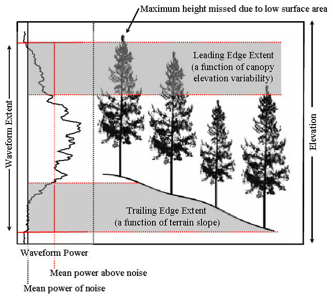
Figure 1. Definition of total waveform, leading and trailing edge extents, and their relationship to forest canopy structure, from Lefsky et al., 2007.
Stratification of Land Cover
The International Geosphere Biosphere Program (IGBP) classification scheme was used from the 2004 500-m Moderate Resolution Imaging Spectroradiometer (MODIS) global land cover (MOD12Q1) data (Justice et al., 1998), to stratify cover types within sub-biome. The 2004 500-m MCD12Q1 IGBP product defined forests as vegetation > 2 m in height (Friedl et al., 2002).
For a consistent biome-level analysis, land area was evaluated that was associated with ecoregions contained within the boreal forest biome of Eurasia. The boreal land area, and its component ecoregions, was defined by the World Wildlife Fund's (WWF) ecoregion map of the world (Olson et al., 2001). These ecoregions, along with satellite-based land cover data, were used to create land cover strata, whereby the same land cover falling in different ecoregions was distinguished as unique strata. This stratum designation allowed for further refinement of land cover data and provided a means of grouping ground plots and LiDAR data.
The data were incorporated into models to provide biomass estimations across all strata and included variance estimations. Refer to Neigh et al. (2013) for additional details.
6. Data Access:
These data are available through the Oak Ridge National Laboratory (ORNL) Distributed Active Archive Center (DAAC).
Contact for Data Center Access Information:
E-mail: uso@daac.ornl.gov
Telephone: +1 (865) 241-3952
7. References:
Denning, A.S., et al. 2005. Science implementation strategy for the North American Carbon Program: A Report of the NACP Implementation Strategy Group of the U.S. Carbon Cycle Interagency Working Group. U.S. Carbon Cycle Science Program, Washington, DC. 68 pp.
Friedl, M. A., McIver, D. K., Hodges, J. C. F., Zhang, X. Y., Muchoney, D., Strahler, A. H., et al. (2002). Global land cover mapping from MODIS: Algorithms and early results. Remote Sensing of Environment, 83, 287–302.
Harding, D. J., and Carabajal, C. C. (2005). ICESat waveform measurements of within-footprint topographic relief and vegetation vertical structure. Geophysical Research Letters, 32, L21S10.
Justice, C. O., Vermote, E., Townshend, J. R. G., Defries, R., Roy, D. P., Hall, D. K., et al. (1998). The Moderate Resolution Imaging Spectroradiometer (MODIS): Land remote sensing for global change research. IEEE Transactions on Geoscience and Remote Sensing, 36, 1228–1249.
Lambert, M. C., Ung, C. H., and Raulier, F. (2005). Canadian national tree aboveground biomass equations. Canadian Journal of Forest Research-Revue Canadienne De Recherche Forestiere, 35, 1996–2018.
Lefsky, M.A., M. Keller, Y. Pang, P.B. De Camargo, and M.O. Hunter. (2007). Revised method for forest canopy height estimation from Geoscience Laser Altimeter System waveforms. Journal of Applied Remote Sensing, 1, 013537-013537-013518.
Lefsky, M., Harding, D., Parker, G., Acker, S., and Gower, S. (2002). LiDAR remote sensing of above-ground biomass in three biomes. Global Ecology and Biogeography, 11, 393–399.
Lefsky , M.A., D. Harding, W.B. Cohen and G.G. Parker. 1999. Surface lidar remote sensing of basal area and biomass in deciduous forests of eastern Maryland, USA. Remote Sensing of the Environment. 67:83-98.
Næsset, E., Gobakken, T., Solberg, S., Gregoire, T. G., Nelson, R., Ståhl, G., et al. (2011). Model-assisted regional forest biomass estimation using LiDAR and InSAR as auxiliary data: A case study from a boreal forest area. Remote Sensing of Environment, 115, 3599–3614.
Neigh, C.S.R., R.F. Nelson, K.J. Ranson, H.A. Margolis, P. M. Montesano, G. Sun, V. Kharuk, E. Naesset, M.A. Wulder, and H.E. Anderson. 2013. Taking stock of circumboreal forest carbon with ground measurements, airborne and spaceborne LiDAR. Remote Sensing of Environment,137, 276-287 doi:10.1016/j.rse.2013.06.019.
Nelson, R. (2010). Model effects on GLAS-based regional estimates of forest biomass and carbon. International Journal of Remote Sensing, 31, 1359–1372.
Olson, D. M., Dinerstein, E., Wikramanayake, E. D., Burgess, N. D., Powell, G. V. N., Underwood, E. C., et al. (2001). Terrestrial ecoregions of the worlds: A new map of life on Earth. Bioscience, 51, 933–938.
Selkowitz, D. J., and Stehman, S. V. (2011). Thematic accuracy of the National Land Cover Database (NLCD) 2001 land cover for Alaska. Remote Sensing of Environment, 115, 1401–1407.
Stahl, G., Holm, S., Gregoire, T. G., Gobakken, T., Næsset, E., and Nelson, R. (2011). Model-based inference for biomass estimation in a LiDAR sample survey in Hedmark County, Norway. Canadian Journal of Forest Research-Revue Canadienne De Recherche Forestiere, 41, 96–107.
Sun, G., Ranson, K. J., Kimes, D. S., Blair, J. B., and Kovacs, K. (2008). Forest vertical structure from GLAS: An evaluation using LVIS and SRTM data. Remote Sensing of Environment, 112, 107–117.
Yong, P., Sun, G. Q., and Li, Z. Y. (2004). Effects of forest spatial structure on large footprint LiDAR waveform. IGARSS 2004: IEEE International Geoscience and Remote Sensing Symposium Proceedings, Vols. 1–7. (pp. 4738–4741).
Wofsy, S.C., and R.C. Harriss. 2002. The North American Carbon Program (NACP). Report of the NACP Committee of the U.S. Interagency Carbon Cycle Science Program. U.S. Global Change Research Program, Washington, DC. 56 pp.
Zwally, H., R. Schutz, C. Bentley, J. Bufton, T. Herring, J. Minster, J. Spinhirne, and R. Thomas. 2014. GLAS/ICESat L2 Global Land Surface Altimetry Data. Version 34. [indicate subset used]. Boulder, Colorado USA: NASA National Snow and Ice Data Center Distributed Active Archive Center. http://dx.doi.org/10.5067/ICESAT/GLAS/DATA227.
Zwally, H., R. Schutz, C. Bentley, J. Bufton, T. Herring, J. Minster, J. Spinhirne, and R. Thomas. 2011. GLAS/ICESat L1A Global Altimetry Data. Version 33. Boulder, Colorado USA: NASA National Snow and Ice Data Center Distributed Active Archive Center. http://dx.doi.org/10.5067/ICESAT/GLAS/DATA121.