Documentation Revision Date: 2024-04-25
Dataset Version: 1
Summary
This dataset includes seven data files in comma-separated values (*.csv) format and two in GeoJSON (*.geojson) format.
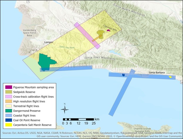
Figure 1: Map of the SHIFT study area in Santa Barbara County, California showing the Jack and Laura Dangermond Preserve, Sedgwick Reserve, and Figueroa Mountain sampling areas and AVIRIS-NG coverage by coastal and terrestrial flightlines. The base map distinguishes public lands (green shaded) from private lands. Figure from Chadwick et al. (in review).
Citation
Queally, N., F.W. Davis, K.D. Chadwick, C. Ade, L. Anderegg, Y. Angel, B. Baker, I. Boving, R.K. Braghiere, P. Brodrick, P. Campbell, J. Cryer, K.C. Cushman, P.D. Dao, A. Dibartolo, R. Eckert, K. Grant, B. Heberlein, M. Johnson, J. Joutras, K. Kerr, C. Kibler, M. Klope, K. Kovach, A. Kreisberg, P. Lovegreen, A.J. Maguire, C. Mcmahon, K. Miner, C. Nickles, F. Ochoa, J.P. Ocón, A. Ongjoco, E. Ordway, M. Park, R. Pavlick, A.M. Raiho, D.A. Roberts, C.M. Saiki, F.D. Schneider, K. Thompson, P. Townsend, E. Vermeer, C. Villanueva-Weeks, N. Vinod, T. Zheng, K. Zumdahl, and D.S. Schimel. 2024. SHIFT: Vegetation Plot Characterization, Santa Barbara County, CA, 2022. ORNL DAAC, Oak Ridge, Tennessee, USA. https://doi.org/10.3334/ORNLDAAC/2295
Table of Contents
- Dataset Overview
- Data Characteristics
- Application and Derivation
- Quality Assessment
- Data Acquisition, Materials, and Methods
- Data Access
- References
Dataset Overview
This dataset contains vegetation plot locations, descriptions, fractional cover, and sample identifier information from surveys conducted as part of the 2022 NASA Surface Biology Geology (SBG) High Frequency Time series (SHIFT) campaign. Surveys took place from 2022-02-23 to 2022-09-27 at the Jack and Laura Dangermond Preserve, Sedgwick Reserve, and Carpinteria Salt Marsh Reserve, which are located in Santa Barbara County, California, USA. This project collected field data contemporaneously with weekly flights of the NASA Airborne Visible-Infrared Imaging Spectrometer-Next Generation (AVIRIS-NG) facility instrument over the study areas. Plot information includes: plot tree subform, species lists, plot description, plot samples characterization, and plot location and contextual information. Related data packages contain additional biogeochemical, reflectance, and foliar data.
Project: Surface Biology and Geology High-Frequency Time Series (SHIFT)
The Surface Biology and Geology (SBG) High Frequency Time Series (SHIFT) was an airborne and field campaign during February to May, 2022, with a follow up activity for one week in September, in support of NASA's SBG mission. Its study area included a 640-square-mile (1,656-square-kilometer) area in Santa Barbara County and the coastal Pacific waters. The primary goal of the SHIFT campaign was to collect a repeated dense time series of airborne Visible to ShortWave Infrared (VSWIR) airborne imaging spectroscopy data with coincident field measurements in both inland terrestrial and coastal aquatic areas, supported in part by a broad team of research collaborators at academic institutions. The SHIFT campaign leveraged NASA's Airborne Visible-Infrared Imaging Spectrometer-Next Generation (AVIRIS-NG) facility instrument to collect approximately weekly VSWIR imagery across the study area. The SHIFT campaign 1) enables the NASA SBG team to conduct traceability analyses related to the science value of VSWIR revisit without relying on multispectral proxies, 2) enables testing algorithms for consistent performance over seasonal time scales and end-to-end workflows including community distribution, and 3) provides early adoption test cases to SHIFT application users and incubate relationships with basic and applied science partners at the University of California Santa Barbara Sedgwick Reserve and The Nature Conservancy's Jack and Laura Dangermond Preserve.
Related Publication:
Chadwick, K.D., F. Davis, K.R. Miner, R. Pavlick, M. Reynolds, P.A. Townsend, P.G. Brodrick, C. Ade, J. Allen, L. Anderegg, Y. Angel, I. Boving, K.B. Byrd, P. Campbell, L. Carberry, K.C. Cavanaugh, K. Easterday, R. Eckert, M. Gierach, K. Gold, E. Hestir, F. Huemmrich, M. Klope, R. Kokaly, P. Lovegreen, K. Luis, C. McMahon, N. Nidzieko, F. Ochoa, A. Jiselle Ongjoco, E. Ordway, M. Pascolini-Campbell, N. Queally, D.A. Roberts, C.M. Saiki, F.D. Schneider, A.N. Shiklomanov, G.D. Silva, J. Snyder, M. Thornton, A. Trugman, N. Vinod, T. Zheng, D.M. Avouris, B. Baker, L. Baskaran, T. Bell, M. Berg, M. Bernas, N. Bohn, R.K. Braghiere, Z. Breuer, A.J. Brooks, N. Burkard, K. Cawse-Nicholson, J. Chapman, J. Chazaro-Haraksin, J. Cryer, K.C. Cushman, K. Dahlin, P.D. Dao A. DiBartolo, M. Eastwood, C. Elder, A. Giordani, K. Grant, R.O. Green, A. Hanson, B. Heberlein, M. Helmlinger, S. Hook, D. Jensen, E. Johnson, M. Johnson, M. Kiper, C. Kibler, J.Y. King, K.R. Kovach, A. Kreisberg, D. Lacey, E. Lang, C. Lee, A.M. Lopez, B. Lopez Barreto, A. Maguire, E. Marsh, C. Miller, D.M.T. Nguyen, C. Nickles, J.P. Ocón, E.P. Papen, M. Park, B. Poulter, A. Raiho, P. Reim, T.H. Robinson, F.E. Romero Galvan, E. Shafron, S. Stroschein, N.C. Taylor, D.R. Thompson, K. Thompson, C. Tye, J. Van Beek, C. Vanden Heuvel, J. Vellanoweth, E. Vermeer, C. Villanueva-Weeks, K. Zumdahl, D. Schimel. Unlocking Ecological Insights from Subseasonal Visible-to-Shortwave Infrared Imaging Spectroscopy: The SBG High Frequency Time Series (SHIFT) Campaign. [Manuscript in review.]
Related Datasets:
Chadwick, K.D., N. Queally, T. Zheng, J. Cryer, C. Vanden Heuvel, C. Villanueva-Weeks, C. Ade, L. Anderegg, Y. Angel, B. Baker, I. Boving, R.K. Braghiere, P. Brodrick, P. Campbell, K.C. Cushman, F. Davis, P.D. Dao, A. Dibartolo, R. Eckert, K. Grant, B. Heberlein, M. Johnson, J. Joutras, C. Kibler, M. Klope, K. Kovach, A. Kreisberg, P. Lovegreen, A.J. Maguire, C. Mcmahon, K. Miner, C. Nickles, F. Ochoa, J.P. Ocón, A. Ongjoco, E. Ordway, M. Park, R. Pavlick, A.M. Raiho, D.A. Roberts, D.S. Schimel, F.D. Schneider, K. Thompson, P. Townsend, E. Vermeer, N. Vinod, and K. Zumdahl. 2023. SHIFT Photosynthetic and Leaf Traits, Santa Barbara County, 2022. ORNL DAAC, Oak Ridge, Tennessee, USA. https://doi.org/10.3334/ORNLDAAC/2233.
- Provides leaf images and measurements of leaf traits (area, wet weight, dry weight, leaf mass per area, leaf water content) and leaf pigments (chlorophyll) and species information
Queally, N., F.W. Davis, K.D. Chadwick, C. Ade, L. Anderegg, Y. Angel, B. Baker, L. Baskaran, I. Boving, R.K. Braghiere, P. Brodrick, P. Campbell, J. Cryer, K.C. Cushman, P.D. Dao, A. Dibartolo, R. Eckert, K. Grant, B. Heberlein, M. Johnson, J. Joutras, K. Kerr, C. Kibler, M. Klope, K. Kovach, A. Kreisberg, P. Lovegreen, A.J. Maguire, C. Mcmahon, K. Miner, C. Nickles, F. Ochoa, J.P. Ocón, A. Ongjoco, E. Ordway, M. Park, R. Pavlick, A.M. Raiho, D.A. Roberts, C.M. Saiki, F.D. Schneider, K. Thompson, P. Townsend, E. Vermeer, C. Villanueva-Weeks, N. Vinod, T. Zheng, K. Zumdahl, and D.S. Schimel. 2024. SHIFT: Vegetation Plot Photos, Santa Barbara, CA, USA, 2022. ORNL DAAC, Oak Ridge, Tennessee, USA. https://doi.org/10.3334/ORNLDAAC/2334
- Provides photographs of the plots where field vegetation sampling was conducted during the 2022 NASA Surface Biology Geology (SBG) High Frequency Time series (SHIFT) campaign
Zheng, T., N. Queally, K.D. Chadwick, J. Cryer, P. Reim, P. Townsend, E. Marsh, M. Berg, Z. Breuer, N. Burkard, A. Hanson, E. Johnson, D. Lacey, A. Lee, L. Pfau, I. Shifrin, B. Skalitzky, S. Stroschein, J. Van beek, C. Vanden heuvel, and A. Williams. 2023. SHIFT: Reflectance Measurements for Dried and Ground Leaf Materials. ORNL DAAC, Oak Ridge, Tennessee, USA. https://doi.org/10.3334/ORNLDAAC/2244
- Provides spectra of dried and ground leaf material
Data Characteristics
Spatial Coverage: Data were collected from plots within Dangermond Preserve, Sedgwick Reserve, and Carpinteria Salt Marsh Reserve, all within Santa Barbara County. California, USA
Spatial Resolution: Point measurements
Temporal Coverage: 2022-02-23 to 2022-09-27
Temporal Resolution: One-time measurements
Study Areas: Latitude and longitude are given in decimal degrees.
| Site | Westernmost Longitude | Easternmost These are the coordinates of the Longitude | Northernmost Latitude | Southernmost Latitude |
|---|---|---|---|---|
| Dangermond Preserve | -120.50 | -120.35 | 34.58 | 34.44 |
| Sedgwick Reserve | -120.07 | -120.01 | 34.74 | 34.68 |
| Carpinteria Salt Marsh Reserve | -119.55 | -119.52 | 34.41 | 34.39 |
Data File Information
This dataset includes seven data files in comma-separated values (*.csv) format and two in GeoJSON (*.geojson) format. GeoJSON files contain polygons of the vegetation plot sites. Comma-separated value files contain vegetation plot survey results and associated metadata.
- SHIFT_vegetation_life_form_codes.csv contains a key for determining life forms (Lifeform_code).
- SHIFT_vegetation_plot_event_list.csv contains metadata associated with the vegetation survey in each plot.
- SHIFT_vegetation_quadrat_tallies.csv contains vegetation survey data conducted using quadrats. Quadrat tallies were conducted only in grassland plots.
- SHIFT_vegetation_sample_list.csv contains information related to plants that had a physical sample collected. Physical samples were collected for species with at least 20% cover within a plot.
- SHIFT_vegetation_shift_plots.csv contains plot location information and summaries of the vegetation survey results within that plot.
- SHIFT_vegetation_species_list.csv contains species characteristics and creates a linkage between ‘Species_or_type’ and ‘Lifeform_code’
- SHIFT_vegetation_tree_subform.csv contains additional fields specific to ‘Plot_event_ID’s where trees were observed
Missing values: Files use -9999 for numeric fields and “N/A’ in other field types.
Comma-separated value files were designed to be able to be integrated with one another and with other SHIFT datasets. A crosswalk figure is available in Figure 2 below.
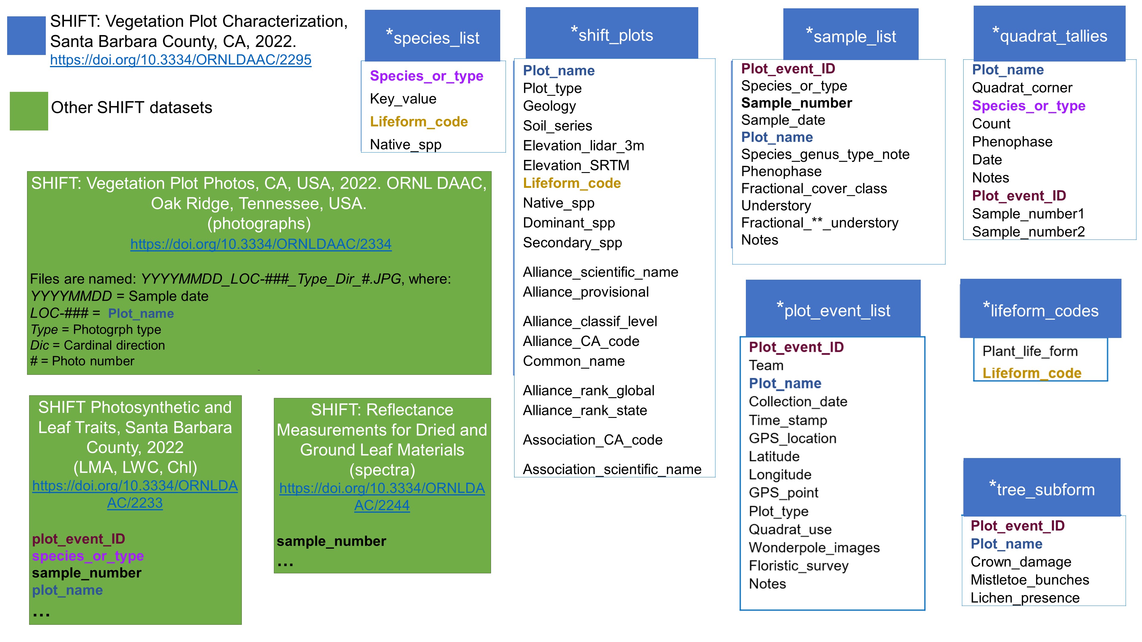
Figure 2. Variable crosswalk for SHIFT vegetation plot survey data.
Table 1. Data Dictionary for SHIFT_vegetation_plot_event_polygons.geojson and SHIFT_vegetation_Ordway_SHIFT_polygons.geojson
| Variable | Units | Description |
|---|---|---|
| Plot_name | Plot name shift_plots.csv | |
| ID | Plot event identifier from plot_event_list.csv | |
| Sample_date | YYYY-MM-DD | Sample Date |
Table 2. Data Dictionary for SHIFT_vegetation_life_form_codes.csv
| Variable | Units | Description |
|---|---|---|
| Plant_life_form | Plant life form | |
| Lifeform_code | Lifeform code |
Table 3. Data Dictionary for SHIFT_vegetation_plot_event_list.csv
| Variable | Units | Description |
|---|---|---|
| Plot_event_ID | Plot event identifier (unique) | |
| Team | Team identifier | |
| Plot_name | Plot name from shift_plots.csv | |
| Collection_date | M/DD/YYYY | Date of plot sampling |
| GPS_location | Decimal Degrees | Latitude and longitude of plot in decimal degrees |
| Latitude | Decimal Degrees | Latitude |
| Longitude | Decimal Degrees | Longitude |
| GPS_point | Spatial positioning of GPS point within plot | |
| Plot_type | Indicates quadrat use (Yes or No) | |
| Quadrat_use | Wonderpole images present (Yes or No) | |
| Wonderpole_images | Floristic survey completed (Yes or No) | |
| Notes | Notes |
Table 4. Data Dictionary for SHIFT_vegetation_quadrat_tallies.csv
| Variable | Units | Description |
|---|---|---|
| Plot_name | Plot name from shift_plots.csv | |
| Quadrat_corner | Corner of the plot that quadrat was placed within (NE, NW, SE, SW) | |
| Species_or_type | Species or type indentifier. From species_list.csv | |
| Count | Integer count of the number of quadrat cells in which this species or type was found. Quadrat contained 50 cells in total. | |
| Phenophase | Phenophase observed | |
| Date | YYYY-MM-DD | Date |
| Notes | Notes | |
| Plot_event_ID | Plot event identifier from plot_event_list.csv | |
| Sample_number1 | Sample number from sample_list.csv | |
| Sample_number2 | Sample number from sample_list.csv in the event that multiple samples were taken associated with this tally entry |
Table 5. Data Dictionary for SHIFT_vegetation_sample_list.csv
| Variable | Units | Description |
|---|---|---|
| Plot_event_ID | Plot event ID from plot_event_list.csv | |
| Species_or_type | Species or type identifier. From species_list.csv | |
| Sample_number | Sample number, linked to trait data in (K.D. Chadwick et al, 2023; Zheng et al, 2023) | |
| Sample_data | YYYY-MM-DD | Sample date |
| Plot_name | Name of plot, prefix indicates sampling region, from shift_plots.csv | |
| Species_genus_type_note | Species/genus/type note | |
| Phenophase | Phenophase - if multiple are indicated, samples were collected from "full leaf out foliage and any other specified phenophases ("Seeds", "Flowers") are noted for reference. In cases where only "Seeds" or "Flowers" are indicated, the sample consists of these components. | |
| Fractional_cover_class | Percentage of fractional coverage in the following intervals: 1-10%, 10-25%, 25-50%, 50-75%, 75-100% | |
| Understory | Indicates if sampling is from understory (Yes or No) | |
| Fractional_coverage_class_understory | Fractional cover class of the understory. Percentage of fractional coverage in the following intervals: 1-10%, 10-25%, 25-50%, 50-75%, 75-100% | |
| Notes | Notes |
Table 6. Data Dictionary for SHIFT_vegetation_shift_plots.csv
| Variable | Units | Description |
|---|---|---|
| Plot_name | Plot name from shift_plots.csv | |
| Plot_type | Plot type (grassland, scrub, shrub) or individual name (tree). Unique, does not vary through time | |
| Geology | Geology codes are abbreviations for geological formations and other mapping classes used by Tom Dibblee for mapping surficial geology of southern California | |
| Soil_series | Soil Series code from Soil Survey Geographic Database (SSURGO) | |
| Elevation_lidar_3m | LIDAR elevation | |
| Elevation_SRTM | Shuttle Radar Topography Mission (SRTM) elevation | |
| Lifeform_code | Lifeform from life_form_codes.csv | |
| Native_spp | Native species | |
| Dominant_spp | Dominant species | |
| Secondary_spp | Secondary species | |
| Alliance_scientific_name | Alliance scientific name (CNPS, 2022) | |
| Alliance_provisional | Alliance provisional (CNPS, 2022) | |
| Alliance_classif_level | Alliance classification level (CNPS, 2022) | |
| Alliance_CA_code | Alliance CA code (CNPS, 2022) | |
| Common_name | Common name (CNPS, 2022) | |
| Alliance_rank_global | Alliance rank global (CNPS, 2022) | |
| Alliance_rank_state | Alliance rank state (CNPS, 2022) | |
| Association_CA_code | Association CA code (CNPS, 2022) | |
| Association _scientific_name | Association scientific name (CNPS, 2022) |
Table 7. Data Dictionary for SHIFT_vegetation_species_list.csv
| Variable | Units | Description |
|---|---|---|
| Species_or_type | Species or cover type identifier | |
| Key_value | Species key value | |
| Lifeform_code | Lifeform from life_form_codes.csv | |
| Native_spp | Native true=1, false=0 |
Table 8. Data Dictionary for SHIFT_vegetation_tree_subform.csv
| Variable | Units | Description |
|---|---|---|
| Plot_event_ID | Plot event ID from plot_event_list.csv | |
| Plot_name | Plot name from shift_plots.csv | |
| Crown_damage | Percentage of crown damage | |
| Mistletoe_bunches | Count of mistletoe bunches (Arceuthobium campylopodum - Western dwarf mistletoe | |
| Lichen_presence | Percentage of lichen presence |
Application and Derivation
Field sampling activity was designed to collect vegetation and plot characteristic data to coincide with the timing of the weekly AVIRIS-NG flights. The data were collected for the SHIFT campaign to support the SBG mission and to provide information on plant communities over a large region of Santa Barbara County, California.
Quality Assessment
Uncertainty information was not provided.
Data Acquisition, Materials, and Methods
Study sites:
Study sites were located in Santa Barbara County, California to coincide spatiotemporally with weekly AVARIS-NG flights. Sites selected for sampling had high vegetative cover and homogeneous characteristics relative to the immediately surrounding area. In addition, within a sampling area a set of sites were selected that represented a range of species and species assemblages. Grassland and low shrub plots were set up as square, 8-m x 8-m plots with four quadrants. Trees and tall shrubs were set up as the extent of the individual crown. For grassland and low shrub plots, photographs were taken of each quadrant from above using a Wonderpole. For grassland plots alone, fractional cover was assessed in each quadrant using a gridded 0.5-m x 1-m quadrat with 50 cells.
Methodology:
Survey Site Metadata Collection
Vegetation and plot characteristic data were sampled three days a week in order to match with that week’s AVIRIS-NG flights. A field team of 45 individuals (around 10 per day) organized into 2-3 teams conducted physical sample collection of a mixture of grass, shrub, and tree plots. Teams assessed fractional cover using quadrats and conducted a floristic survey of all species occurring in the plot. Teams collected high-accuracy GPS data using a Trimble Geo 7x, with an accuracy of ~25 cm, for the plot center or a designated corner of the plot. The plot perimeter was collected using a lower-accuracy GPS-enabled iPad with TouchGIS, typically accurate to within 3-15 m depending on canopy openness (see reference). Each sample received a unique sample number that was linked to the unique plot name.
The number of sampling sites was determined based on the amount of canopy samples desirable for sufficient ground truth data for developing statistical models to map foliar traits. Based on sample sizes in successful canopy-scale trait modeling projects (Singh et al.; K. Dana Chadwick et al.; Wang et al.), as well as phenologically-informed modeling efforts (Chlus and Townsend), The goal was to survey 500 plots, prioritizing both diversity of species and phenological variation within species.
Sites selected for sampling had high vegetative cover and homogeneous characteristics relative to the immediately surrounding area. In addition, within a sampling area sites were selected that represented a range of species and species assemblages in order to capture a wide range across the multi-dimensional trait space. In total 485 unique sites were surveyed, with revisits to 129 of them. These collections took place over the course of three months, from late February 2022 - Late May 2022, with an additional week of collections (and accompanying flight) in September 2022. In all, this resulted in 1218 foliar samples and sites with documented species cover, provided here.
For all plots, a unique plot name was designated and date, time, GPS point (using in the CSV files) and polygon (used the GeoJSON files), plot type (e.g., tree) were recorded. Also, a landscape photograph of the plot was taken. A floristic survey was conducted, in which all present species were noted in the plot and their phenophase and relative cover % as seen from above. For species that could not be identified in the field, a voucher sample and identifying photographs were taken to later be identified by Dr. Frank Davis, La Kretz Center director and botanist. With the improved orthorectificaiton of the AVIRIS-NG data for the SHIFT project and the flight altitude designed to achieve 5-m x 5-m pixels, grassland and low shrub plots were set up as square, 8-m x 8-m plots with four quadrants. Trees and tall shrub plots were set up as the extent of the individual crown, which covered at least an 8-m x 8-m area. For grassland and low shrub plots, photographs were taken of each quadrant from above using a Wonderpole. For grassland plots alone, fractional cover was also assessed in each quadrant using a gridded 0.5-m x 1-m quadrat with 50 cells. For tree plots, photogaphs of the overstory and understory were taken. If a species within a plot covered at least 20% of the plot (estimated as seen from the plane), a physical sample was collected. If flowers, fruit (seeds), or senescent vegetation met this same threshold, those materials were collected as a separate sample. Additional “bulk” samples were collected at grassland plots, which consisted of four random clippings of foliar sample from across the plot, to later compare to plot-aggregated trait estimates. Each sample received a unique sample number (‘Sample_number’) that were linked to the unique plot name (‘Plot_name’). Note: The photographs mentioned above are available in Queally et al (2024).
Species taxonomy and nomenclature are according to Baldwin and Goldman (2012). Vegetation Alliance and Association identities are according to the Manual of California Vegetation (CNPS 2022). Species were identified from the following sources:
- Baldwin, B. G., & Goldman, D. H. (Eds.). 2012. The Jepson manual: vascular plants of California. Univ of California Press.
- CNPS. 2022. A Manual of California Vegetation, Online Edition. http://www.cnps.org/cnps/vegetation/; searched on February 1, 2022. California Native Plant Society, Sacramento, CA.
Survey site polygon generation
Based on the high-accuracy GPS data and the GPS perimeters collected during the survey, polygons that represent the spatial extent of each sampling site were developed and are presented in GeoJSON format in this datset.
For the grassland and low shrub plots, GPS points were collected from one designated corner, and the 8m x 8m perimeter was walked to define the polygon. Perimeter coordinates were collected using a GPS-enabled iPad with TouchGIS software. For tall shrubs and trees, the polygons are the extent of the crown for the individual that was sampled. This method allows for the selection of all pixels that are associated with the plot, rather than selecting an arbitrary distance from the GPS point that was collected. A team of SHIFT participants manually assessed each plot shapefile in post-processing and aligned the plot extent using the SHIFT imagery from the associated flight date for that particular plot to ensure the extraction of the correct pixels for each date. As such, the precise location of these shapefiles may be offset from other data products and should be evaluated accordingly.
Data Access
These data are available through the Oak Ridge National Laboratory (ORNL) Distributed Active Archive Center (DAAC).
SHIFT: Vegetation Plot Characterization, Santa Barbara County, CA, 2022
Contact for Data Center Access Information:
- E-mail: uso@daac.ornl.gov
- Telephone: +1 (865) 241-3952
References
Baldwin, B.G., and D.H. Goldman. (Eds.). 2012. The Jepson manual: vascular plants of California. Univ of California Press.
Chadwick, K.D., F. Davis, K.R. Miner, R. Pavlick, M. Reynolds, P.A. Townsend, P.G. Brodrick, C. Ade, J. Allen, L. Anderegg, Y. Angel, I. Boving, K.B. Byrd, P. Campbell, L. Carberry, K.C. Cavanaugh, K. Easterday, R. Eckert, M. Gierach, K. Gold, E. Hestir, F. Huemmrich, M. Klope, R. Kokaly, P. Lovegreen, K. Luis, C. McMahon, N. Nidzieko, F. Ochoa, A. Jiselle Ongjoco, E. Ordway, M. Pascolini-Campbell, N. Queally, D.A. Roberts, C.M. Saiki, F.D. Schneider, A.N. Shiklomanov, G.D. Silva, J. Snyder, M. Thornton, A. Trugman, N. Vinod, T. Zheng, D.M. Avouris, B. Baker, L. Baskaran, T. Bell, M. Berg, M. Bernas, N. Bohn, R.K. Braghiere, Z. Breuer, A.J. Brooks, N. Burkard, K. Cawse-Nicholson, J. Chapman, J. Chazaro-Haraksin, J. Cryer, K.C. Cushman, K. Dahlin, P.D. Dao A. DiBartolo, M. Eastwood, C. Elder, A. Giordani, K. Grant, R.O. Green, A. Hanson, B. Heberlein, M. Helmlinger, S. Hook, D. Jensen, E. Johnson, M. Johnson, M. Kiper, C. Kibler, J.Y. King, K.R. Kovach, A. Kreisberg, D. Lacey, E. Lang, C. Lee, A.M. Lopez, B. Lopez Barreto, A. Maguire, E. Marsh, C. Miller, D.M.T. Nguyen, C. Nickles, J.P. Ocón, E.P. Papen, M. Park, B. Poulter, A. Raiho, P. Reim, T.H. Robinson, F.E. Romero Galvan, E. Shafron, S. Stroschein, N.C. Taylor, D.R. Thompson, K. Thompson, C. Tye, J. Van Beek, C. Vanden Heuvel, J. Vellanoweth, E. Vermeer, C. Villanueva-Weeks, K. Zumdahl, D. Schimel. Unlocking Ecological Insights from Subseasonal Visible-to-Shortwave Infrared Imaging Spectroscopy: The SBG High Frequency Time Series (SHIFT) Campaign. [Manuscript in review.]
Chadwick, K.D., N. Queally, T. Zheng, J. Cryer, C. Vanden Heuvel, C. Villanueva-Weeks, C. Ade, L. Anderegg, Y. Angel, B. Baker, I. Boving, R.K. Braghiere, P. Brodrick, P. Campbell, K.C. Cushman, F. Davis, P.D. Dao, A. Dibartolo, R. Eckert, K. Grant, B. Heberlein, M. Johnson, J. Joutras, C. Kibler, M. Klope, K. Kovach, A. Kreisberg, P. Lovegreen, A.J. Maguire, C. Mcmahon, K. Miner, C. Nickles, F. Ochoa, J.P. Ocón, A. Ongjoco, E. Ordway, M. Park, R. Pavlick, A.M. Raiho, D.A. Roberts, D.S. Schimel, F.D. Schneider, K. Thompson, P. Townsend, E. Vermeer, N. Vinod, and K. Zumdahl. 2023. SHIFT Photosynthetic and Leaf Traits, Santa Barbara County, 2022. ORNL DAAC, Oak Ridge, Tennessee, USA. https://doi.org/10.3334/ORNLDAAC/2233.
Chadwick, K.D., P.G. Brodrick, K. Grant, T. Goulden, A. Henderson, N. Falco, H. Wainwright, K.H. Williams, M. Bill, I. Breckheimer, E.L. Brodie, H. Steltzer, C.F. R. Williams, B. Blonder, J. Chen, B. Dafflon, J. Damerow, M. Hancher, A. Khurram, J. Lamb, C.R. Lawrence, M. McCormick, J. Musinsky, S. Pierce, A. Polussa, M. Hastings Porro, A. Scott, H.W. Singh, P.O. Sorensen, C. Varadharajan, B. Whitney, and K. Maher. 2020. Integrating airborne remote sensing and field campaigns for ecology and Earth system science. Methods in Ecology and Evolution 11:1492–1508. https://doi.org/10.1111/2041-210X.13463
Chlus, A., and P.A. Townsend. 2022. Characterizing seasonal variation in foliar biochemistry with airborne imaging spectroscopy. Remote Sensing of Environment 275:113023. https://doi.org/10.1016/j.rse.2022.113023
CNPS (California Native Plant Society). 2022. A Manual of California Vegetation, Online Edition. http://www.cnps.org/cnps/vegetation; searched on February 1, 2022. California Native Plant Society, Sacramento, CA.
Queally, N., F.W. Davis, K.D. Chadwick, C. Ade, L. Anderegg, Y. Angel, B. Baker, L. Baskaran, I. Boving, R.K. Braghiere, P. Brodrick, P. Campbell, J. Cryer, K.C. Cushman, P.D. Dao, A. Dibartolo, R. Eckert, K. Grant, B. Heberlein, M. Johnson, J. Joutras, K. Kerr, C. Kibler, M. Klope, K. Kovach, A. Kreisberg, P. Lovegreen, A.J. Maguire, C. Mcmahon, K. Miner, C. Nickles, F. Ochoa, J.P. Ocón, A. Ongjoco, E. Ordway, M. Park, R. Pavlick, A.M. Raiho, D.A. Roberts, C.M. Saiki, F.D. Schneider, K. Thompson, P. Townsend, E. Vermeer, C. Villanueva-Weeks, N. Vinod, T. Zheng, K. Zumdahl, and D.S. Schimel. 2024. SHIFT: Vegetation Plot Photos, Santa Barbara County, CA, USA, 2022. ORNL DAAC, Oak Ridge, Tennessee, USA. https://doi.org/10.3334/ORNLDAAC/2334
Singh, A., S.P. Serbin, B.E. McNeil, C.C. Kingdon, and P.A. Townsend. 2015. Imaging spectroscopy algorithms for mapping canopy foliar chemical and morphological traits and their uncertainties. Ecological Applications 25:2180–2197. https://doi.org/10.1890/14-2098.1
Wang, Z., A. Chlus, R. Geygan, Z. Ye, T. Zheng, A. Singh, J.J. Couture, J. Cavender-Bares, E.L. Kruger, and P.A. Townsend. 2020. Foliar functional traits from imaging spectroscopy across biomes in eastern North America. New Phytologist 228:494–511. https://doi.org/10.1111/nph.16711
Zheng, T., N. Queally, K.D. Chadwick, J. Cryer, P. Reim, P. Townsend, E. Marsh, M. Berg, Z. Breuer, N. Burkard, A. Hanson, E. Johnson, D. Lacey, A. Lee, L. Pfau, I. Shifrin, B. Skalitzky, S. Stroschein, J. Van beek, C. Vanden heuvel, and A. Williams. 2023. SHIFT: Reflectance Measurements for Dried and Ground Leaf Materials. ORNL Distributed Active Archive Center. https://doi.org/10.3334/ORNLDAAC/2244