Summary:
This data set provides two products that were derived from the recently published North American Carbon Program (NACP) Regional Synthesis 1-degree terrestrial biosphere model (TBM) and inverse model (IM) outputs (Gridded 1-deg Observation Data and Biosphere and Inverse Model Outputs, Wei et al., 2013).
The first product is the aggregation of the standardized gridded 1-degree TBM and IM outputs to the Greenhouse Gas (GHG) inventory zones as defined for North America (United States, Canada, and Mexico). Depending on the data availability, the monthly/yearly Net Ecosystem Exchange (NEE), Net Primary Production (NPP), Total Vegetation Carbon (VegC), Heterotrophic Respiration (Rh), and Fire Emissions (FE) outputs from the 22 TBM and 7 IM models were aggregated from the 1-degree resolution gridded format to the inventory zones and then, further divided into Forest Lands, Crop Lands, and Other Lands sectors within each inventory zone based on the 1-km resolution GLC2000 land cover map (GLC2000, 2003).
The second product is the North American national GHG inventories on the scale of inventory zones which contain estimated land-atmosphere exchange of CO2 (NEE) in forest lands, crop lands, and other lands sectors. NEE estimates were synthesized from inventory-based data on productivity, ecosystem carbon stock change, and harvested product stock change, and additional information from national-level GHG inventories of the United States, Canada, and Mexico including EPA (2011) and Environment Canada (2011).
An additional summary file of annual mean NEE (2000-2006) is provided for both land sectors and reporting zones in North America and was created by combining the aggregated model output and the national GHG database and is provided.
The aggregated monthly and yearly model output data and the national GHG inventories data are available in comma separated value (*.csv) format files.
Also provided are detailed inventory zone spatial data as an ESRI Shapefile. Included are zone names, boundaries, and zone and land cover type area attributes. For mapping convenience, the inventory zones shapefile was merged with 1-km forest, crop, and other lands masks to create a 1-km resolution reference data file that was converted to GeoTIFF format. The GeoTIFF defines to which inventory zone and land cover type each 1-km grid cell belongs.
This document provides detailed information about the content, format, and processing procedures of these two data products. Detailed descriptions of the TBMs and IMs can be found in a separate companion document: NACP Regional Synthesis - Description of Observations and Models.
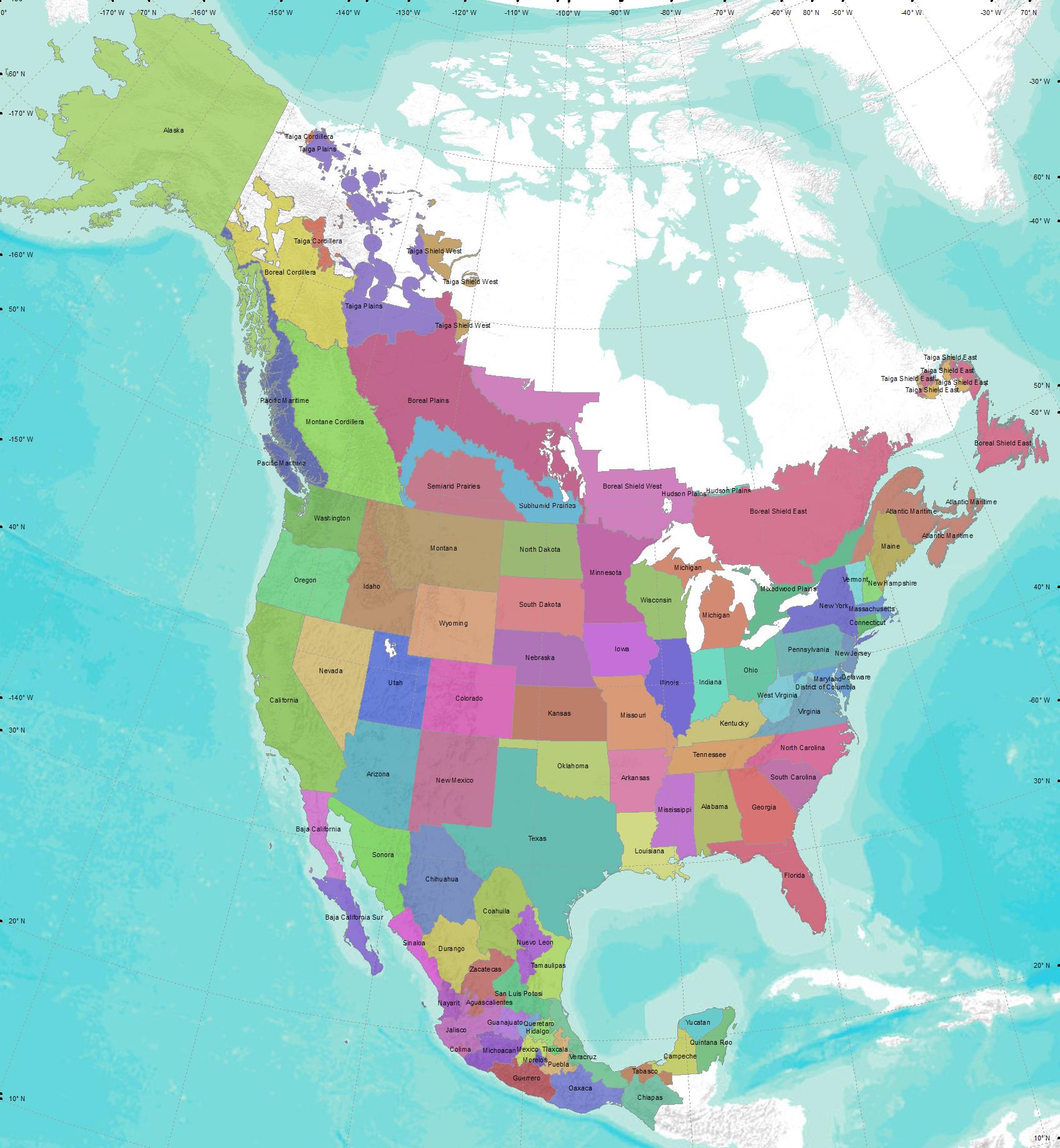
Figure 1. North American inventory zones map.
This data set is related to two other processed regional data sets (i.e., NACP Regional: Gridded 1-deg Observation Data and Biosphere and Inverse Model Outputs; and NACP Regional: Supplemental Gridded Observations, Biosphere and Inverse Model Outputs); and to the originally-submitted NACP Regional: Original Observation Data and Biosphere and Inverse Model Outputs. The data set was also used in the model-inventory comparison activities of the NACP Regional Synthesis.
This data set was compiled by the Modeling and Synthesis Thematic Data Center (MAST-DC). MAST-DC was a component of the NACP (www.nacarbon.org) designed to support NACP by providing data products and data management services needed for modeling and synthesis activities. The overall objective of MAST-DC was to provide data management support to NACP investigators and agencies performing modeling and synthesis activities. The products were used in the model-inventory comparison activities of the NACP Regional Synthesis.
Data and Documentation Access:
Get Data: http:daac.ornl.gov/cgi-bin/dsviewer.pl?ds_id=1179
Companion Documentation for this Data Set:
- Regional-Description_of_Observations_and_Models.pdf
- Regional-Standardized_Inventory_Zones.pdf
- NACP_Model_Metadata_Survey_Results.pdf
- NACP_Model_Characteristics.pdf
Model Characteristics Overview and References: NACP_Model_Characteristics.pdf
Related Data Products:
NACP Regional: Original Observation Data and Biosphere and Inverse
Model Outputs
NACP Regional: Gridded 1-deg Observation Data and Biosphere and Inverse Model Outputs [http:daac.ornl.gov/cgi-bin/dsviewer.pl?ds_id=1157]
NACP Regional: Supplemental
Gridded Observation, Biosphere and Inverse Model Outputs [http:daac.ornl.gov/cgi-bin/dsviewer.pl?ds_id=1158]
Data Citation:
Cite this data set as follows:
Wei, Y., D.J. Hayes, M.M. Thornton, W.M. Post, R.B. Cook, P.E. Thornton, A.R. Jacobson, D.N. Huntzinger, T.O. West, L.S. Heath, B. McConkey, G. Stinson,W. Kurz, B. de Jong, I. Baker, J. Chen, F. Chevallier, F.M. Hoffman, A. Jain, R. Lokupitiya, D.A. McGuire, A. Michalak, G.G. Moisen, R.P. Neilson, P. Peylin, C. Potter, B. Poulter, D. Price, J. Randerson, C. Rodenbeck, H. Tian, E. Tomelleri, G. van der Werf, N. Viovy, J. Xiao, N. Zeng, and M. Zhao. 2013. NACP Regional: National Greenhouse Gas Inventories and Aggregated Gridded Model Data. Data set. Available on-line [http://daac.ornl.gov] from Oak Ridge National Laboratory Distributed Active Archive Center, Oak Ridge, Tennessee, USA http://dx.doi.org/10.3334/ORNLDAAC/1179
Table of Contents:
- 1 Data Set Overview
- 2 Data Description
- 3 Applications and Derivation
- 4 Quality Assessment
- 5 Acquisition Materials and Methods
- 6 Data Access
- 7 References
1. Data Set Overview:
Project: North American Carbon Program (NACP)
The NACP (Denning et al., 2005; Wofsy and Harriss, 2002) is a multidisciplinary research program to obtain scientific understanding of North America's carbon sources and sinks and of changes in carbon stocks needed to meet societal concerns and to provide tools for decision makers. Successful execution of the NACP has required an unprecedented level of coordination among observational, experimental, and modeling efforts regarding terrestrial, oceanic, atmospheric, and human components. The program has relied upon a rich and diverse array of existing observational networks, monitoring sites, and experimental field studies in North America and its adjacent oceans. It is supported by a number of different federal agencies through a variety of intramural and extramural funding mechanisms and award instruments.
NACP and MAST-DC organized several synthesis activities to evaluate and inter-compare biosphere model outputs and observation data at local to continental scales for the time period of 2000 through 2005. The synthesis activities have included three component studies, each conducted on different spatial scales and producing numerous data products: (1) site-level analyses that examined process-based model estimates and observations at over 30 AmeriFlux and Fluxnet-Canada tower sites across North America; (2) a regional, mid-continent intensive study centered in the agricultural regions of the United States and focused on comparing inventory-based estimates of net carbon exchange with those from atmospheric inversions; and (3) a regional and continental synthesis evaluating model estimates against each other and available inventory-based estimates across North America. A number of other NACP syntheses were conducted, including ones focusing on non-CO2 greenhouse gases, the impact of disturbance on carbon exchange, and coastal carbon dynamics. The Oak Ridge National Laboratory (ORNL) Distributed Active Archive Center (DAAC) is the archive for the NACP synthesis data products.
NACP Regional Synthesis
This data set contains part of the third NACP synthesis product described above: regional analyses. The data products were compiled and used in model-inventory comparison activities.
Table 1. Contributors
| Last Name | First Name | Organization | Role | |
|---|---|---|---|---|
| Wei | Yaxing | ORNL | weiy@ornl.gov | MAST-DC |
| Hayes | Daniel | ORNL | hayesdj@ornl.gov | Synthesis Lead |
| Thornton | Michele M. | ORNL | thorntonmm@ornl.gov | MAST-DC |
| Post | Wilfred M. | University of Tennessee | wmp@ornl.gov | MAST-DC |
| Cook | Robert B. | ORNL | cookrb@ornl.gov | MAST-DC |
| Thornton | Peter E. | ORNL | thorntonpe@ornl.gov | MAST-DC, CLM-CN |
| Jacobson | Andy | NOAA | andy.jacobson@noaa.gov | Synthesis Lead, CarbonTracker |
| Huntzinger | Deborah N. | Northern Arizona University | deborah.huntzinger@nau.edu | Synthesis Lead |
| Baker | Ian | Colorado State University | baker@atmos.colostate.edu | SIB3.1 |
| Chen | Jing | University of Toronto | chenj@geog.utoronto.ca | BEPS |
| Chevallier | Frederic | LSCE | Frederic.Chevallier@lsce.ipsl.fr | LSCE no.2 |
| Hoffman | Forrest | ORNL | forrest@climatemodeling.org | CLM-CASA |
| Jain | Atul | University of Illinois at Urbana-Champaign | jain@atmos.uiuc.edu | ISAM |
| Liu | Shuguang | USGS | sliu@usgs.gov | EC-LUE |
| Lokupitiya | Ravi | Colorado State University | ravi@atmos.colostate.edu | CSU no.1 |
| McGuire | David A. | University of Alaska Fairbanks | ffadm@uaf.edu | TEM6 |
| Michalak | Anna | Stanford University | michalak@stanford.edu | Michigan Geostatistical |
| Moisen | Gretchen G. | USDA Forest Service | gmoisen@fs.fed.us | U.S. Forest Biomass |
| Neilson | Ronald P. | USDA Forest Service | rneilson@fs.fed.us | MC1 |
| Peylin | Philippe | LSCE |
Philippe.Peylin@lsce.ipsl.fr
|
LSCE no.1 |
| Potter | Chris | NASA Ames Research Center | chris.potter@nasa.gov | NASA-CASA |
| Poulter | Ben | Potsdam Institute for Climate Impact Research |
ben.poulter@pik- potsdam.de |
LPJmL |
| Price | David | Canadian Forest Service |
dprice@nrcan.gc.ca |
Can-IBIS |
| Randerson | Jim | University of California Irvine | jranders@uci.edu | CASA-Transcom |
| Rödenbeck | Christian | Max Planck Institute for Biogeochemistry | christian.roedenbeck@bgc-jena.mpg.de | Jena |
| Tian | Hanqin | Auburn University | tianhan@auburn.edu | DLEM |
| Tomelleri | Enrico | Max Planck Institute for Biogeochemistry |
etomell@bgc-jena.mpg.de |
MOD17-plus |
| van der Werf | Guido | University Amsterdam | guido.van.der.werf@falw.vu.nl | CASA-GFEDv2 |
| Viovy | Nicolas | LSCE |
viovy@lsce.ipsl.fr |
ORCHIDEE |
| West | Tristram O. | PNNL |
tristram.west@pnnl.gov |
Crop NPP |
| Xiao | Jingfeng | University of New Hampshire | j.xiao@unh.edu | EC-MOD |
| Zeng | Ning | University of Maryland at College Park | zeng@atmos.umd.edu | VEGAS |
| Zhao | Maosheng | University of Montana | zhao@ntsg.umt.edu | MODIS GPP/NPP |
Table 2 lists all of the models and their corresponding output variables that were aggregated to inventory zones, along with their temporal coverage and resolution. For selected models and output variables, other variables were used to derive the data. For example, the aggregated Veg variable of model CLM-CASA was derived from LEAFC+WOODC+FROOTC, which was comparable to variable TOTVEGC of model CLM-CN or variable TotLivBiom of model MC1. A cell marked with “n/a” means a variable is neither directly available nor derivable from other variables for a model.
Table 2. List of Model and Variables Aggregated to Inventory Zones
| Model | Temporal Coverage* | Temporal Resolution | Variables | ||||||
|---|---|---|---|---|---|---|---|---|---|
| NEE | NPP | Veg | Rh | FE | |||||
| Terrestrial Biosphere Models | CLM-CASA | i01.54 | 2000-2004 | monthly | NEE | NPP | (LEAFC + WOODC + FROOTC) | HR | n/a |
| i01.54_q15 | |||||||||
| i01.55 | |||||||||
| i01.55_q15 | |||||||||
| CLM-CN | i01.56 | 2000-2004 | monthly | NEE | NPP | TOTVEGC | HR | n/a | |
| i01.57_q15 | |||||||||
| ORCHIDEE | 2001-2007 | monthly | CO2FLUX | NPP | n/a | HET_RESP | n/a | ||
| SiB3 | 2000-2005 | monthly | NEE | n/a | n/a | n/a | n/a | ||
| CASA-Transcom | 2002-2003 | monthly | NEE | n/a | n/a | n/a | n/a | ||
| CASA GFed2 | 2000-2005 | monthly | NEEF | n/a | n/a | n/a | CFire (derived from NEEF-NEE) | ||
| NASA-CASA | 2001-2004 | monthly | (-1 * NEP) | NPP | n/a | (NPP – NEP) | n/a | ||
| MC1 | 2000-2007 | monthly | NEE + BioCons | NPP | TotLivBiom | RespH | BioCons | ||
| TEM6 | 2000-2006 | monthly | NCE | NPP | VEGC | RH | (NCE - NEE) | ||
| DLEM | 2000-2005 | monthly | NEE | NPP | TotLivBiom | Rh | n/a | ||
| VEGAS | 2000-2007 | monthly | NEE | NPP | cvege | Rh | cfire | ||
| EC-MOD | 2001-2006 | monthly | NEE | n/a | n/a | n/a | n/a | ||
| MOD17-plus | 2000-2004 | monthly | (GPP – Reco) | n/a | n/a | n/a | n/a | ||
| ISAM | 2000-2007 | monthly | NEE | NPP | n/a | resp | n/a | ||
| BEPS | 2000-2004 | monthly | (-1 * NEP) | NPP | n/a | (NPP - NEP) | n/a | ||
| LPJmL | 2000-2006 | monthly, yearly | NEE (monthly), ANEEF (annually, derived from ANEE+FIRE) | NPP | VEGC (annually) | RH | FIRE (annually) | ||
| Can-IBIS | 2000-2005 | monthly,yearly | NEE (derived from -1*NEP) | NPP | CBiomass (annually) | Rh | n/a | ||
| Inverse Models | UToronto | 2001-2003 | monthly | NEE | n/a | n/a | n/a | n/a | |
| CarbonTracker | 2000-2007 | monthly | NEE | n/a | n/a | n/a | n/a | ||
| LCSE-no1 (Peylin) | 2002-2004 | monthly | NEE | n/a | n/a | n/a | n/a | ||
| JENA (Rodenbeck) | 2000-2007 | monthly | NEE | n/a | n/a | n/a | n/a | ||
| Michigan-Geostatistical | 2000-2001 | monthly | NEE | n/a | n/a | n/a | n/a | ||
| CSU-no1 (MLEF-PCTM) | 2003-2004 | monthly | NE | n/a | n/a | n/a | n/a | ||
| LSCE-no2 (Chevalier) | 2000-2006 | monthly | NEE | n/a | n/a | n/a | n/a | ||
Note: * Only data in and after year 2000 were included in aggregation.
Table 3. Data Product Summary
| Data Set Category | Sub Category | Variables | File Formats |
|---|---|---|---|
| Model Outputs Aggregated to Inventory Zones | Terrestrial Biosphere Model (TBM) Outputs | 5 (NEE, NPP, VegC, Rh, FE) | Comma-Separated-Value (.csv) |
| Inverse Model (IM) Outputs | 1 (NEE) | ||
| GHG Inventory Data | National GHG inventories and the estimation of land-atmosphere exchange of CO2 (NEE) by reporting zone and land sector | 9 (forest area, live biomass C, soil organic matter/non-live, non-soil C, fire CO2 emissions, C removal as harvested products, NPP, HR, C emissions in processing of harvested products, NEE) | |
| NEE (2000-2006) Summary Data | Annual mean NEE (2000-2006) by sectors and zones in North America | 1 (NEE) |
2. Data Description:
Aggregated Model Output
This data set contains two major categories of data:
(1) standardized gridded biosphere model and inverse model outputs aggregated to the inventory zones defined for North America (United States, Canada, and Mexico) and further divided into Forest Lands, Crop Lands, and Other Lands sectors for each inventory zone based on the 1-km resolution GLC2000 land cover map; and
(2) North American national GHG inventories, which contain estimated land-atmosphere exchange of CO2 (NEE) in Forest Lands, Crop Lands, and Other Lands sectors synthesized from inventory-based data on productivity, ecosystem carbon stock change and harvested product stock change.
An additional summary file of annual mean NEE (2000-2006) by both land sectors and reporting zones in North America was created by combining the aggregated model output and the national GHG database and is provided.
The aggregated monthly/yearly model output data and the national GHG inventories data are stored in comma separated value (*.csv) format.
Spatial Data Connection
All the above data files are non-spatial data, but they can be linked to the two auxiliary spatial data files described below for further spatial analysis and mapping purposes. NAZonesFine.shp is a Shapefile that provides detailed inventory zones information, including zone names, boundaries, and associated zone attributes at a spatial scale of 1:15,000,000. NA_Reporting_Zones_Sectors.tif is a 1-km resolution reference zone and sector mask data file in GeoTIFF format that defines to which reporting zone and sector each 1-km grid cell belongs. It was created by merging the North American reporting zones shapefile with land sector masks.
2.1. Spatial Coverage
Site: North America
Site boundaries: (All latitude and longitude given in decimal degrees)
| Site (Region) | Westernmost Longitude | Easternmost Longitude | Northernmost Latitude | Southernmost Latitude |
|---|---|---|---|---|
| North America | -170 | -50 | 84 | 10 |
2.2. Coordinate Reference System
The Coordinate Reference System (CRS) of both auxiliary spatial data files is WGS 84.
Below is its definition in the format of Open Geospatial Consortium Well Know Text (OGC WKT) format:
GEOGCS["WGS 84",
DATUM["WGS_1984",
SPHEROID["WGS 84",6378137,298.257223563,
AUTHORITY["EPSG","7030"]],
AUTHORITY["EPSG","6326"]],
PRIMEM["Greenwich",0,
AUTHORITY["EPSG","8901"]],
UNIT["degree",0.01745329251994328,
AUTHORITY["EPSG","9122"]],
AUTHORITY["EPSG","4326"]]
2.3. Spatial Resolution
The spatial scale for the inventory zone shapefile NAZonesFine.shp is 1:15,000,000. The spatial resolution for the reference zone & sector mask data file is 0.0089285714 degree, or about 1-km.
2.4. Temporal Coverage
Varies (range: 2000-2007)
2.5. Temporal Resolution
Monthly or yearly
2.6. Data File Information
2.6.1. Aggregated Model Output
For each TBM and IM model, a compressed file (model.zip) contains the aggregated output data files, organized by variable, with one data file for each of the monthly and yearly time periods in and after 2000. The output variables and temporal range for each model are listed in Table 2.
Table 4. Terrestrial Biosphere Model Output Data Files
| TBM Output Data Files | IM Output Data Files |
| TBM_BEPS_InventoryZone.zip | IM_CSU-no1_Zone.zip |
| TBM_CASA-GFEDv2_InventoryZone.zip | IM_CarbonTracker_Zone.zip |
| TBM_CASA-Transcom_InventoryZone.zip | IM_JENA_Zone.zip |
| TBM_CLM-CASA_55_Zonal_Monthly.zip | |
| IM_LCSE-no1_Zone.zip | |
| TBM_CLM-CASA_i54_InventoryZone.zip | |
| IM_LCSE-no2_Zone.zip | |
| TBM_CLM-CASA_i54q15_InventoryZone.zip | IM_Michigan-Geostatistical_Zone.zip |
| TBM_CLM-CASA_i55q15_InventoryZone.zip | IM_UToronto_Zone.zip |
| TBM_CLM-CN_56_Zonal_Monthly.zip | |
| TBM_CLM-CN_57q15_Zonal_Monthly.zip | |
| TBM_CLM-CN_Zonal_Monthly.zip | |
| TBM_Can-IBIS_InventoryZone.zip | |
| TBM_DLEM_Zonal_Monthly.zip | |
| TBM_EC-MOD_Zonal_Monthly.zip | |
| TBM_ISAM_Zonal_Monthly.zip | |
| TBM_LPJmL_Zonal_Monthly.zip | |
| TBM_MC1_Zonal_Monthly.zip | |
| TBM_MOD17-plus_Zonal_Monthly.zip | |
| TBM_NASA-CASA_Zonal_Monthly.zip | |
| TBM_ORCHIDEE_Zonal_Monthly.zip | |
| TBM_SiB3-plus_Zonal_Monthly.zip | |
| TBM_TEM6_Zonal_Monthly.zip | |
| TBM_VEGAS2_Zonal_Monthly.zip |
When a compressed file (model.zip) is expanded, the data files are organized by variable and named as follows:
Annual time-step data files are named as: model_variable_YYYY.csv
Monthly time-step data files are named as: model_variable_YYYYMM.csv
Example of Expanded Model Output File: TBM_CLM-CN_Zonal_Monthly.zip
TBM_CLM-CN_Zonal_Monthly/ (there is a subdirectory for each output variable)
NEE/
CLMCN_NEE_2000.csv (annual file, YYYY)
…
CLMCN_NEE_2004.csv
CLMCN_NEE_200001.csv (monthly file, YYYYMM)
…
CLMCN_NEE_200412.csv
NPP/
Rh/
Veg or VegC/
FE/
NEEF/
Note that IM model files only contain NEE data files.
Model Output File Contents:
For each variable, the following information is provided at each annual and monthly time step: a sum and area-weighted average for each zone, the sum of each variable by land cover type (forest, crop, other) for each zone, and the area-weighted average of each variable by land cover type (forest, crop, other) for each zone.
Table 5. Annual Data File Contents:
| Column Name | Units | Description |
|---|---|---|
| OBJECTID | Unique ID of each reporting zone. It can be used to link back to the reporting zone polygons for mapping and spatial analysis. Also, Zone_ID | |
| Zone_ | Name of reporting zone. Also, Zone_Name | |
| SUM_variable* | kgC/year | Sum of variable for forest, crop, and other land cover types for zone. Sum of next three columns. |
| SUM_variable_F | kgC/year | Sum of variable for forest land cover type for zone. |
| SUM_variable_C | kgC/year | Sum of variable for crop land cover type for zone. |
| SUM_ variable_O | kgC/year | Sum of variable for all other land cover types for zone. |
| AVG_variable | kgC/m2/year | Area-weighted average of variable for forest, crop, and other land cover types for zone. |
| AVG_variable_F | kgC/m2_of_forest_area/year | Area-weighted average of variable for forest land cover type for zone. |
| AVG_variable_C | kgC/m2_of_crop_area/year | Area-weighted average of variable for crop land cover type for zone. |
| AVG_variable_O | kgC/m2_of_other_area/year | Area-weighted average of variable for all other land cover types for zone. |
| MODEL_NAME | Model abbreviation/acronym | |
| PERIOD | YYYY | Year reported. |
*variable = NEE, NPP, Rh, VegC**, FE, NEEF
**Note that VegC was reported as a single monthly estimate of biomass -- not the sum of more frequent estimates.
Example Data Records: BEPS_NEE_2000.csv
|
OBJECTID,Zone_,SUM_NEE,SUM_NEE_F,SUM_NEE_C,SUM_NEE_O,AVG_NEE,AVG_NEE_F, AVG_NEE_C,AVG_NEE_O,MODEL_NAME,PERIOD 1,"Aguascalientes",1348576487.9333,354109096.48465,124316331.60469,870151059.8416,0.241047345,0.241495992, 0.258280493,0.238592579,"BEPS","2000" 2,"Alabama",-3469663161.320003,-52290465.266001,-2545006998.444,-872365697.6271,-0.025819, -0.000519, -0.102347,-0.099634,"BEPS","2000" 3,"Alaska",1557942057.51001,4226545721.485,-503947616.85851,-2164656047.252998,0.001032567, 0.010325192, -0.033816,-0.001996,"BEPS","2000" … 37,"Kentucky",-6286697580.731999,-503608786.5066,-5536245211.075,-246843583.1518,-0.060367, -0.008801, -0.124193,-0.105449,"BEPS","2000" 56,"New Jersey",-4621521636.3857,-3553303595.4253,-403854192.2452,-664363848.7137,-0.234434, -0.267431, -0.179307,-0.159149,"BEPS","2000" 72,"San Luis Potosi",23016515438.107,7922971766.1432,10299937853.608,4793605818.3542,0.359743892, 0.493990662, 1.169769434,0.122484361,"BEPS","2000" |
Table 6. Monthly Data File Contents:
| Column Name | Units | Description |
|---|---|---|
| OBJECTID | Unique ID of each reporting zone. It can be used to link back to the reporting zone polygons for mapping and spatial analysis. Also, Zone_ID | |
| Zone_ | Name of reporting zone. Also, Zone_Name | |
| SUM_variable* | kgC/month | Sum of variable for forest, crop, and other land cover types for zone. Sum of next three columns. |
| SUM_variable_F | kgC/month | Sum of variable for forest land cover type for zone. |
| SUM_variable_C | kgC/month | Sum of variable for crop land cover type for zone. |
| SUM_variable_O | kgC/month | Sum of variable for all other land cover types for zone. |
| AVG_variable | kgC/m2/month | Area-weighted average of variable for forest, crop, and other land cover types for zone. |
| AVG_variable_F | kgC/m2_of_forest_area/month | Area-weighted average of variable for forest land cover type for zone. |
| AVG_variable_C | kgC/m2_of_crop_area/month | Area-weighted average of variable for crop land cover type for zone. |
| AVG_variable_O | kgC/m2_of_other_area/month | Area-weighted average of variable for all other land cover types for zone. |
| MODEL_NAME | Model abbreviation/acronym |
*variable = NEE, NPP, Rh, VegC**, FE, NEEF
**Note that VegC was reported as a single monthly estimate of biomass -- not the sum of more frequent estimates.
Example Data Records: LPJmL_NPP_200412.csv
|
OBJECTID,Zone_,SUM_NEE,SUM_NEE_F,SUM_NEE_C,SUM_NEE_O,AVG_NEE,AVG_NEE_F, AVG_NEE_C,AVG_NEE_O,MODEL_NAME,PERIOD 1,"Aguascalientes",-188405989.211,-50187718.2739,-16245868.144,-121972402.793, -0.033676, -0.034227,-0.033753,-0.033444 2,"Alabama",2700373282.88,2079147028.96,447472522.485,173753731.432, 0.020094261,0.020634001, 0.017995067,0.01984454 3,"Alaska",-2039038892.45,-629978804.87,-58795085.4363,-1350265002.14, -0.001351,-0.001539, -0.003945,-0.001245 … 95,"Wyoming",-596649117.106,-226724409.814,-6400282.72015,-363524424.572, -0.002346,-0.003803,-0.002213,-0.001895 96,"Yucatan",-297105626.192,-222049975.169,-59293206.5953,-15762444.4289, -0.007848, -0.007363,-0.008712,-0.017647 97,"Zacatecas",-1712269243.9,-304987190.751,-29052579.5864,-1378229473.57, -0.022886,-0.023377,-0.030178,-0.022665 |
2.6.2. GHG Inventories and NEE
GHG inventories, which contain estimated land-atmosphere exchange of CO2 (NEE) in Forest Lands, Crop Lands, and Other Lands sectors synthesized from inventory-based data on productivity, ecosystem carbon stock change and harvested product stock change, and additional information from national-level GHG inventories of the United States, Canada, and Mexico.
For ease of comparison, the descriptions below of the *.csv data files are grouped by Forest Lands, Crop Lands, and Other Lands rather than by country.
Table 7. National GHG Inventory Data Files
| FILE NAMES | |
|---|---|
| COMPRESSED FILE NAMES | UNCOMPRESSED DATA FILE NAMES |
| Inventory_CAN.zip | Inventory_CAN_Crop.csv |
| Inventory_CAN_Forest.csv | |
| Inventory_CAN_Other.csv | |
| Inventory_MEX.zip | Inventory_MEX_Forest.csv |
| Inventory_MEX_Other.csv | |
| Inventory_USA.zip | Inventory_USA_Crop.csv |
| Inventory_USA_Forest.csv | |
| Inventory_USA_Other.csv | |
2.6.3. Attributes of Forest Lands GHG Inventories and NEEF
Canada Forest Lands: Table 8 lists the major components of GHG inventories and the estimation of land-atmosphere exchange of CO2 (NEEF) by Canada reporting zone in forest lands sector.
Table 8. Attributes of Canada Forest Lands GHG Inventories
| Attribute | Attribute Column Name | Units | Description |
|---|---|---|---|
| Zone ID | Zone_ID | Unique ID of each reporting zone. It can be used to link back to the reporting zone polygons for mapping and spatial analysis. | |
| SectorZone ID | SectorZone_ID | Unique ID of each reporting zone and land sector combination. It can be used to link back to reference land sector mask data for mapping and spatial analysis. | |
| Zone Name | Zone_Name | Name of reporting zone. | |
| Forest Area | Forest_Area | km2 | Area of forest in each reporting zone. |
| ΔLiveC | dLiveC | TgC yr-1 | Carbon stock change in live biomass pools |
| ΔDOM | dDOM | TgC yr-1 | Carbon stock changes in soil organic matter and in non-live, non-soil pools (standing dead, litter, coarse woody debris) |
| Fire (C) | FireC | TgC yr-1 | Fire emissions (carbon in all forms) |
| HR | HCRemoved | TgC yr-1 | Total C removed from the stand as harvests in the Managed Forest sector of each reporting zone |
| NPP | NPP | TgC yr-1 | Net Primary Productivity |
| Rh | Rh | TgC yr-1 | Heterotrophic Respiration |
| Fire (CO2) | FireCO2 | TgC yr-1 | Fire emissions (carbon in CO2 only) |
| HE | HCEmitted | TgC yr-1 | The amount of C emitted from the processing of harvested products within the forest sector = -0.3*HR |
| NEEF | NEE | TgC yr-1 | ΔLiveC + ΔDOM - (Fire (C ) - Fire (CO2)) + HR + HE = NPP + Rh + Fire (CO2) + HE |
U.S. Forest Lands: Table 9 lists the major components of GHG inventories and the estimation of land-atmosphere exchange of CO2 (NEEf) by US States in forest lands sector.
Table 9. Attributes of US Forest Lands GHG Inventories
| Attribute | Attribute Column Name | Units | Description |
|---|---|---|---|
| Zone ID | Zone_ID | Unique ID of each reporting zone. It can be used to link back to the reporting zone polygons for mapping and spatial analysis. | |
| SectorZone ID | SectorZone_ID | Unique ID of each reporting zone and land sector combination. It can be used to link back to reference land sector mask data for mapping and spatial analysis. | |
| Zone Name | Zone_Name | Name of reporting zone. | |
| Forest Area | Forest_Area | km2 | Area of forest in each reporting zone. |
| ΔLiveC | dLiveC | TgC yr-1 | Carbon stock change in live biomass pools |
| ΔDOM | dDOM | TgC yr-1 | Carbon stock changes in soil organic matter and in non-live, non-soil pools (standing dead, litter, coarse woody debris) |
| HR | HCRemoved | TgC yr-1 | Total C removed from the stand as harvested products in each reporting zone |
| HE | HCEmitted | TgC yr-1 | The amount of C emitted from the processing of harvested products within the forest sector = -0.3*HR |
| NEEF | NEE | TgC yr-1 | NEEF = ΔLive + ΔDOM + HR + HE |
Mexico Forest Lands: Table 10 lists the major components of GHG inventories and the estimation of land-atmosphere exchange of CO2 (NEEf) by Mexico States in forest lands sector.
Table 10. Attributes of Mexico Forest Lands GHG Inventories
| Attribute | Attribute Column Name | Units | Description |
|---|---|---|---|
| Zone ID | Zone_ID | Unique ID of each reporting zone. It can be used to link back to the reporting zone polygons for mapping and spatial analysis. | |
| SectorZone ID | SectorZone_ID | Unique ID of each reporting zone and land sector combination. It can be used to link back to reference land sector mask data for mapping and spatial analysis. | |
| Zone Name | Zone_Name | Name of reporting zone. | |
| Forest Area | Forest_Area | km2 | Area of forest in each reporting zone. |
| ΔLiveLUC | Biomass_Conversion | TgC yr-1 | Carbon stock change in live biomass pools due to forest land use conversion |
| ΔSoilLUC | dSoilC | TgC yr-1 | Carbon stock change in soil organic matter pools due to forest land use conversion |
| ΔLiveABND | Abandonment | TgC yr-1 | Carbon stock change in live biomass pools due to biomass increment on forest land regenerating after agricultural abandonment |
| ΔLiveMNGD | Fuelwood+Uptake | TgC yr-1 | Carbon stock change in live biomass pools due to biomass increment and fuelwood harvest in managed forest land |
| Total NEE | Total_NEE | TgC yr-1 | Total Net Ecosystem Exchange from forest land |
2.6.4. Attributes of Crop Lands GHG Inventories and NEEc
Canada Crop Lands: Table 11 lists the major components of GHG inventories and the estimation of land-atmosphere exchange of CO2 (NEEc) by Canada reporting zone in crop lands sector.
Table 11. Attributes of Canada Crop Lands GHG Inventories
| Attribute | Attribute Column Name | Units | Description |
|---|---|---|---|
| Zone ID | Zone_ID | Unique ID of each reporting zone. It can be used to link back to the reporting zone polygons for mapping and spatial analysis. | |
| SectorZone ID | SectorZone_ID | Unique ID of each reporting zone and land sector combination. It can be used to link back to reference land sector mask data for mapping and spatial analysis. | |
| Zone Name | Zone_Name | Name of reporting zone. | |
| Crop Area | Crop_Area | km2 | Area of crop in each reporting zone. |
| NPP | NPP | TgC yr-1 | Crop Net Primary Productivity |
| HR | Harvest | TgC yr-1 | Total C removed as harvested crop products in each reporting zone |
| ΔSOILC | dSoilC | TgC yr-1 | Carbon stock change in soil organic matter pools in agricultural land |
| NEEC | NEE | TgC yr-1 | NEE = HR + ΔSOILC |
US Crop Lands: Table 12 lists the major components of GHG inventories and the estimation of land-atmosphere exchange of CO2 (NEEc) by US States in crop lands sector.
Table 12. Attributes of US Crop Lands GHG Inventories
| Attribute | Attribute Column Name | Units | Description |
|---|---|---|---|
| Zone ID | Zone_ID | Unique ID of each reporting zone. It can be used to link back to the reporting zone polygons for mapping and spatial analysis. | |
| SectorZone ID | SectorZone_ID | Unique ID of each reporting zone and land sector combination. It can be used to link back to reference land sector mask data for mapping and spatial analysis. | |
| Zone Name | Zone_Name | Name of reporting zone. | |
| Crop Area | Crop_Area | km2 | Area of crop in each reporting zone. |
| NPP | NPP | TgC yr-1 | Crop Net Primary Productivity |
| HR | Harvest | TgC yr-1 | Total C removed as harvested crop products in each reporting zone |
| ΔSOILC | dSoilC | TgC yr-1 | Carbon stock change in soil organic matter pools in agricultural land |
| NEEC | NEE | TgC yr-1 | NEE = HR + ΔSOILC |
2.6.5. Attributes of Other Lands GHG Inventories and NEEo
Canada Other Lands: Table 13 lists the major components of GHG inventories and the estimation of land-atmosphere exchange of CO2 (NEEo) by Canada reporting zone in other lands sector.
Table 13. Attributes of Canada Other Lands GHG Inventories
| Attribute | Attribute Column Name | Units | Description |
|---|---|---|---|
| Zone ID | Zone_ID | Unique ID of each reporting zone. It can be used to link back to the reporting zone polygons for mapping and spatial analysis. | |
| SectorZone ID | SectorZone_ID | Unique ID of each reporting zone and land sector combination. It can be used to link back to reference land sector mask data for mapping and spatial analysis. | |
| Zone Name | Zone_Name | Name of reporting zone. | |
| AO | Other_Area | km2 | Area represented in the Other Lands sector: the Total Reporting Zone Area minus Inventory Forest Area minus Inventory Crop Area |
| PopH | Population | 103 | Human population (thousand persons) in each reporting zone estimated by overlaying reporting zone boundaries on census units containing year 2006 population estimates from Statistics Canada (www.statcan.gc.ca) |
| CH | Human_Crop_Consumption | TgC yr-1 | Human crop consumption and CO2 emissions from human respiration estimated using per capita consumption (61.6 kg C yr-1) and respiration (54.0) rates from the U.S. data ([West et al., 2009]) |
| EH | Human_CO2_Respiration | TgC yr-1 | |
| EL-CH4 | Livestock_CH4_Emissions | TgC yr-1 | Livestock (cattle and swine) methane emissions from Statistics Canada 2006 Census of Agriculture |
| EL | Livestock_CO2_Emissions | TgC yr-1 | Estimated livestock CO2 emissions; the column total is equal to the national total HR adjusted for the net crop harvest export out of the country (27%*), minus national total human crop consumption and total C emitted as CH4 from livestock; the column total is distributed proportional to C emitted as CH4 from livestock in each reporting zone; *national-level crop harvest imports vs. exports is based on cash value, from the Canadian Socio-Economic Information Management System (Statistics Canada) |
| EF | Forest_Product_CO2_Emissions | TgC yr-1 | Estimated CO2 emissions from decay of forest products; the column total is equal to the national total emissions from HWPE which is distributed proportional to human population in each reporting zone |
| NEEG | NEE_Grasslands | TgC yr-1 | NEE for grasslands estimated by multiplying the average grassland sink per area from the U.S. data (2.1 g C m-2 yr-1) by the "other" land area in each reporting zone |
| NEES | NEE_Settlements | TgC yr-1 | NEE for settled areas estimated by multiplying the average settlements sink per capita from the U.S. data (95.6 kg C per capita yr-1) by the human population in each reporting zone |
| NEEO | Total_NEE_Other_Lands | TgC yr-1 | NEEO = EH + EL + EF + NEEG + NEES |
U.S. Other Lands: Table 14 lists the major components of GHG inventories and the estimation of land-atmosphere exchange of CO2 (NEEo) by US States in other lands sector.
Table 14. Attributes of US Other Lands GHG Inventories
| Attribute | Attribute Column Name | Units | Description |
|---|---|---|---|
| Zone ID | Zone_ID | Unique ID of each reporting zone. It can be used to link back to the reporting zone polygons for mapping and spatial analysis. | |
| SectorZone ID | SectorZone_ID | Unique ID of each reporting zone and land sector combination. It can be used to link back to reference land sector mask data for mapping and spatial analysis. | |
| Zone Name | Zone_Name | Name of reporting zone. | |
| AO | Other_Area | km2 | Area represented in the Other Lands sector: the Total Reporting Zone Area minus Inventory Forest Area minus Inventory Crop Area (average area years 2000 - 2006) |
| PopH | Population | 103 | Human population (thousand persons) is the average state population between 2000 and 2006, estimates from U.S. Census Bureau [2009] |
| CH | Human_Crop_Consumption | TgC yr-1 | For human consumption of crop products , there is a consistent respiration-to-consumption multiplier (1.14) across all age/gender classes in Table 1 of West et al., [2009], which was applied to the data on human respiration. |
| EH | Human_CO2_Respiration | TgC yr-1 | |
| EL-CH4 | Livestock_CH4_Emissions | TgC yr-1 | Livestock methane emissions from enteric fermentation from the USDA Greenhouse Gas Inventory [2008] |
| EL | Livestock_CO2_Emissions | TgC yr-1 | Estimated livestock CO2 emissions; the column total is equal to the national total crop harvest (HR from Table A5), adjusted for the net crop harvest export out of the country (HCPIMP – HCPEXP = -46.7 TgC yr-1between 2000 and 2006*), minus national total human crop consumption and total C emitted as CH4 from livestock; the column total is distributed proportional to C emitted as CH4 from livestock in each reporting zone; *national-level crop harvest imports vs. exports is based on volume converted to dry-weight biomass carbon using data in USDA Economic Research Service (2010)."Foreign Agricultural Trade of the United States (FATUS)" [2010] http://www.ers.usda.gov/data/fatus/ |
| EF | Forest_Product_CO2_Emissions | TgC yr-1 | Estimated CO2 emissions from decay of forest products; the column total is equal to the national total emissions from HWP; the column total is distributed proportional to human population in each reporting zone |
| NEEG | NEE_Grasslands | TgC yr-1 | NEE for grasslands estimated by distributing the annual, national-level grassland sink estimates from the U.S. Environmental Protection Agency Greenhouse Gas Inventory [2010] proportional to the area of the Other Land sector in each reporting zone |
| NEES | NEE_Settlements | TgC yr-1 | NEE for settled areas estimated by distributing the annual, national-level settlements / other sink estimates from the U.S. Environmental Protection Agency Greenhouse Gas Inventory [2010] proportional to the human population in each reporting zone |
| NEEO | Total_NEE_Other_Lands | TgC yr-1 | NEEO = EH + EL + EF + NEEG + NEES |
Mexico Other Lands: Table 15 lists the major components of GHG inventories and the estimation of land-atmosphere exchange of CO2 (NEEo) by Mexico States in other lands sector.
Table 15. Attributes of Mexico Other Lands GHG Inventories
| Attribute | Attribute Column Name | Units | Description |
|---|---|---|---|
| Zone ID | Zone_ID | Unique ID of each reporting zone. It can be used to link back to the reporting zone polygons for mapping and spatial analysis. | |
| SectorZone ID | SectorZone_ID | Unique ID of each reporting zone and land sector combination. It can be used to link back to reference land sector mask data for mapping and spatial analysis. | |
| Zone Name | Zone_Name | Name of reporting zone. | |
| AO | Forest_Area | km2 | Area of forest in each reporting zone. |
| ΔLiveLUC | Biomass_Conversion | TgC yr-1 | Carbon stock change in live biomass pools due to non-forest land use conversion |
| ΔSoilLUC | dSoilC | TgC yr-1 | Carbon stock change in soil organic matter pools due to non-forest land use conversion |
| ΔLiveABND | Abandonment | TgC yr-1 | Carbon stock change in live biomass pools due to biomass increment on non-forest land regenerating after agricultural abandonment |
| ΔLiveMNGD | Fuelwood+Uptake | TgC yr-1 | Carbon stock change in live biomass pools due to biomass increment and fuelwood emissions in managed non-forest land |
| Total NEE | Total_NEE | TgC yr-1 | Total Net Ecosystem Exchange from forest land |
2.7. Annual Mean NEE (2000-2006) by Sectors and Zones in North America
Annual mean NEE (2000-2006) summary data by both land sectors and reporting zones in North America (NEE_Zones_Sectors_Mean_2000-2006.csv) was created by combining the aggregated model output and the national GHG database. This NEE summary data can be used for model-inventory comparison purpose directly or be linked with the reference raster data (NA_Reporting_Zones_Sectors.tif) for mapping purpose. Table 16 describes the fields included in the NEE summary data.
Table 16. Attributes of NEE summary data
| Attribute | Attribute Column Name | Units | Description |
|---|---|---|---|
| Sector Zone ID | Zone_ID | Unique ID for each sector-zone combination in the pattern of “NXY”, see section 4 for details | |
| Sector | Sector | Sector type: forest, crop, or other | |
| Zone Name | Zone_Name | Name of reporting zone | |
| Country | Country | Country | |
| NEE from Forward Model | NEE_Forward | g C m-2 yr-1 | Annual mean NEE (2000-2006) from mean of multiple forward models |
| NEE from Inverse Model | NEE_Inverse | g C m-2 yr-1 | Annual mean NEE (2000-2006) from mean of multiple inverse models |
| NEE from GHG Inventory | NEE_Inventory | g C m-2 yr-1 | Annual mean NEE (2000-2006) from national GHG database |
Example Data Records: NEE_Zones_Sectors_Mean_2000-2006.csv
|
Sector_Zone_ID,Sector,Zone_Name,Country,NEE_Forward,NEE_Inverse,NEE_Inventory 101,Forest Land,Aguascalientes,Mexico,4.80,16.52,13.78 102,Forest Land,Alabama,United States,-62.36,-114.35,-138.29 103,Forest Land,Alaska,United States,-10.36,-4.85,-59.48 … 395,Other Land,Wisconsin,United States,-71.98,-99.84,313.25 396,Other Land,Wyoming,United States,0.48,-34.85,11.98 397,Other Land,Yucatan,Mexico,-46.67,-1.12,-26.39 398,Other Land,Zacatecas,Mexico,3.67,-5.90,-8.69 |
2.8. Auxiliary Files
Detailed inventory zones information, including zone names, boundaries, and associated zone attributes are defined in ESRI Shapefile NAZonesFine.shp. File NAZonesFine.shp is described in Section 3 of the companion file, Regional-Standardized Inventory Zones.pdf. The following inventory zones attributes are included in the shapefile:
• Zone (string): Name of the state or reporting zone
• Country (string): The country to which the zone belongs
• SUM_Area (double): Area of the state or reporting zone (in square meters)
• SUM_AreaF (double): Area of forest land cover type within each Zone (in square meters)
• SUM_AreaC (double): Area of crop land cover type
within each Zone (in square meters)
• SUM_AreaO (double): Area of “other” land cover type within each Zone (in square meters)
File NA_Reporting_Zones_Sectors.tif is described in Section 4 of the companion file, Regional-Standardized Inventory Zones.pdf. For the purpose of creating spatial maps as shown in Fig. 5 of Hayes et al. (2012), the North American reporting zones shapefile was merged with masks to create a 1km resolution reference raster data file (NA_Reporting_Zones_Sectors.tif) to describe which reporting zone and sector each 1km grid cell belongs to. The values in the reference raster data are 3-digit numbers following the pattern of “NXY”. If “N” is 1, it means the grid cell belongs to the forest land sector. Value “2” and “3” indicate the crop and “other” land sectors, repectively. “XY” is a 2-digit number representing the ID of reporting zones, as listed in Table 19 below. For example, a grid cell with value 141 means that 1km grid cell belongs to the forest sector and Maryland, U.S.
Table 17. Auxiliary Files
| COMPRESSED FILE NAME | FILE NAME | DESCRIPTION |
|---|---|---|
| NAZonesFine.zip | NAZonesFine.shp | Detailed inventory zones information, including zone names, boundaries, and associated zone attributes at a spatial scale of 1:15,000,000 |
| NA_Reporting_Zones_Sectors.zip | North American reporting zones shapefile merged with 1-km forest, crop, and other lands masks to create a 1-km resolution reference raster data file to describe to which reporting zone and sector each 1-km grid cell belongs. |
2.9. Companion File Information
Table 18. Companion Files
| FILE NAME | DESCRIPTION |
|---|---|
| Regional-Description_of_Observations_and_Models.pdf | Overview of observation measurement data and biosphere and inverse models, including descriptions, sources, contacts, and a comprehensive reference list |
| NACP_Model_Characteristics.pdf | Overview of process descriptions in participating ecosystem or forward models and boundary conditions and driver data used in participating ecosystem or forward models with a comprehensive reference list |
| NACP_Model_Metadata_Survey_Results.pdf | Metadata for Forward (Ecosystem) Model Intercomparison: Site Model Data Comparison and Regional Model Data Comparison: Survey Results |
| Regional-Standardized_Inventory_Zones.pdfs | Provides a description of the aggregation process, inventory zones, and mapping methods. |
3. Data Application and Derivation:
This data product contributes to a multidisciplinary research program to obtain scientific understanding of North America's carbon sources and sinks and of changes in carbon stocks needed to meet societal concerns and to provide tools for decision makers. The data were generated as part of an NACP regional and continental synthesis to evaluate and inter-compare models and observation measurements across North America.
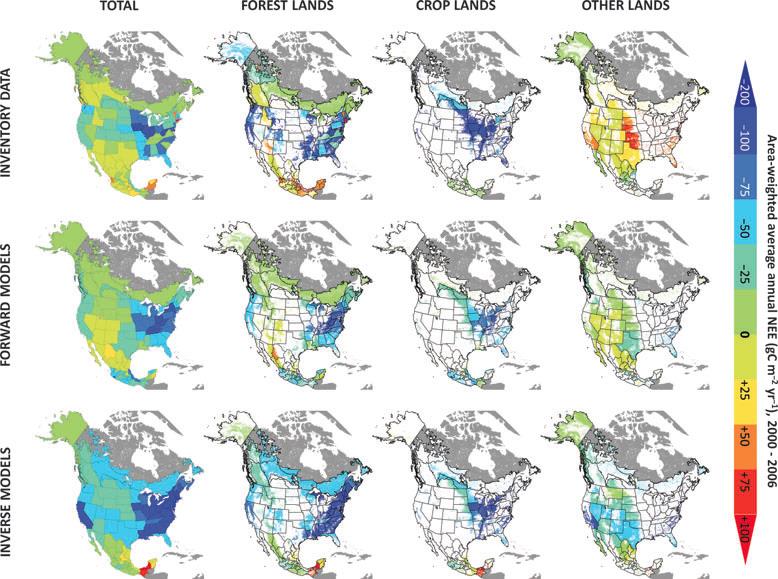
Figure 2. Mean area-weighted average annual NEE (g C m-2 yr-1), 2000–2006 for the Forest Lands, Crop Lands and Other Lands sectors, along with all land (total), in each reporting zone, from inventory-based estimates against mean results from the sets of terrestrial biosphere (forward) models and inverse models. (source: Figure 5 in Hayes, et al., 2012)
4. Quality Assessment:
This study (1) created a set of modeled carbon flux variables (NEE, NPP, VegC, Rh, and Fire Emissions) at the inventory-zone scale by aggregating model results at 1-degree spatial resolution and (2) developed an approach for estimating NEE using inventory-based information over North America for a recent 7-year period (ca. 2000–2006). The approach notably retains information on the spatial distribution of NEE, or the vertical exchange between land and atmosphere of all non-fossil fuel sources and sinks of CO2, while accounting for lateral transfers of forest and crop products as well as eventual emissions.
The GHG inventory-based results were derived from, and so are generally consistent with, recent inventory-based updates of the carbon budgets reported for Canada forests, U.S. forests and agriculture, and the agriculture and forest sector in Mexico. The new information provided in this study comes from the combination of those national- and sector-specific estimates into a continental-scale analysis, while using a novel conceptual model to estimate land-atmosphere exchange of CO2 at the sub-national scale. As a result, the inventory-based data and the methodology used in this study suggest considerable spatial variability in NEE estimates across sectors and reporting zones (Figure 1). The spatial patterns are driven both by the estimated direct, vertical surface fluxes, as well as the lateral transfer of carbon between sectors in the form of harvested products.
The inventory-based estimates of NEE were compared with results from a suite of terrestrial biosphere and atmospheric inversion models. The study used ‘off-the-shelf’ model simulations without a consistent set of driver forcing data or simulation protocols and other recently published studies. These simulations and studies served as a pre-cursor to more formal model inter-comparison activities that will follow this study.
The mean model estimates from both the terrestrial biosphere and inverse models suggest a much stronger overall North American sink than the inventory-based estimate. Yet model estimates generally do follow similar spatial patterns as the inventory-based data where the strongest sinks are found in US forests on the east and west coasts and in croplands of the midcontinent, with a smaller source from the tropical area of southern Mexico. However, the model vs inventory differences are mostly in the magnitude of the estimates.
The wide range in the land surface flux estimates is related to a number of factors, but most generally because of the different methodologies used to develop estimates of carbon stocks and flux, and the uncertainties inherent in each approach:
• Biomass inventories provide valuable constraints on changes in the size of carbon pools over years to decades. However, dynamics and fluxes can be under-sampled or missed altogether (e.g., inventory sampling can produce reliable estimates of biomass, but other carbon pools, such as litter and soil C stocks, may not have been sampled at the same intensity in all areas. Inventory-based modeling can be used to estimate growth and disturbance impacts, but does not yet provide full capability in partitioning the forcing brought about by non-disturbance factors. On the other hand, inventory and commerce data sets can often be used to quantify the storage, emissions and/or lateral movement of carbon in product pools, which are typically not well characterized in modeling approaches.
• TBMs can be used to simulate the dynamics of multiple ecosystem components. However, TBMs contain substantial uncertainty because of the sheer number of often poorly understood underlying processes simulated. They also vary widely in the data used to drive them, in the particular processes simulated, and in their level of detail.
• IM analyses provide constraints on estimates of land-atmosphere carbon exchange at a detailed temporal resolution, relying on the strong diurnal and seasonal cycles in CO2 concentration in the observations. However, these estimates are associated with large uncertainties from the limited density of observation networks, uncertainty in the transport models, and errors in the inversion process.
In summary, this study highlights the differences in three general scaling approaches to NEE (inventory, forward TBMs, and inverse modeling), and by comparing and evaluating their estimates several strengths and weaknesses emerge (Table 18). For additional information, consult Hayes et al. (2012).
Table 19. A comparison of the strengths and weaknesses of alternative NEE scaling approaches (inventory-based, IMs and TBMs (Source: Hayes et al., 2012).
| Inventory-based | Atmospheric Inversion Models (IM) | Terrestrial Biosphere Models (TBM) | |
|---|---|---|---|
| Strengths | Employs a large number of repeated biomass measurements | Assimilates measurements of atmospheric CO2 concentration | Processes are represented so attribution is possible |
| Allows estimation of product related C sources | Employs atmospheric mass balance | Sensitive to interannual variation in climate | |
| Many opportunities for validation | |||
| Weaknesses | Not all C pools are measured | Transport model uncertainty | Many inputs, each with their own uncertainty |
| Potential under-sampling | Limited number of CO2 measurements | Many parameters, each with their own uncertainty | |
| Limited attribution ability | Low spatial resolution | Spatial resolution may not resolve management scale disturbances | |
| Missing NEE of unmanaged ecosystems | Limited attribution ability | ||
| Poorly resolved temporally |
5. Data Acquisition Materials and Methods:
5.1. Inventory Zones
The NACP standardized-gridded model output data were aggregated onto inventory zones in order to be compared with inventory-based national GHG data. The inventory zones for North America are defined as states for the United States and Mexico and ecoregion-based managed forest reporting zones for Canada. The definition of inventory zones for North America is consistent between the aggregated standardized-gridded model output data and the national GHG data. Figure 1 shows the map for all 97 inventory zones in North America and Table 19 lists the zone IDs and names.
Table 20. North American Inventory Zones
| No | Zone ID | Zone Name | Country |
|---|---|---|---|
| 1 | 1 | Aguascalientes | Mexico |
| 2 | 2 | Alabama | United States |
| 3 | 3 | Alaska | United States |
| 4 | 4 | Arizona | United States |
| 5 | 5 | Arkansas | United States |
| 6 | 6 | Atlantic Maritime | Canada |
| 7 | 7 | Baja California | Mexico |
| 8 | 8 | Baja California Sur | Mexico |
| 9 | 9 | Boreal Cordillera | Canada |
| 10 | 10 | Boreal Plains | Canada |
| 11 | 11 | Boreal Shield East | Canada |
| 12 | 12 | Boreal Shield West | Canada |
| 13 | 13 | California | United States |
| 14 | 14 | Campeche | Mexico |
| 15 | 15 | Chiapas | Mexico |
| 16 | 16 | Chihuahua | Mexico |
| 17 | 17 | Coahuila | Mexico |
| 18 | 18 | Colima | Mexico |
| 19 | 19 | Colorado | United States |
| 20 | 20 | Connecticut | United States |
| 21 | 21 | Delaware | United States |
| 22 | 22 | District of Columbia | United States |
| 23 | 23 | Distrito Federal | Mexico |
| 24 | 24 | Durango | Mexico |
| 25 | 25 | Florida | United States |
| 26 | 26 | Georgia | United States |
| 27 | 27 | Guanajuato | Mexico |
| 28 | 29 | Guerrero | Mexico |
| 29 | 30 | Hidalgo | Mexico |
| 30 | 31 | Hudson Plains | Canada |
| 31 | 32 | Idaho | United States |
| 32 | 33 | Illinois | United States |
| 33 | 34 | Indiana | United States |
| 34 | 35 | Iowa | United States |
| 35 | 36 | Jalisco | Mexico |
| 36 | 37 | Kansas | United States |
| 37 | 38 | Kentucky | United States |
| 38 | 39 | Louisiana | United States |
| 39 | 40 | Maine | United States |
| 40 | 41 | Maryland | United States |
| 41 | 42 | Massachusetts | United States |
| 42 | 43 | Mexico | Mexico |
| 43 | 44 | Michigan | United States |
| 44 | 45 | Michoacan | Mexico |
| 45 | 46 | Minnesota | United States |
| 46 | 47 | Mississippi | United States |
| 47 | 48 | Missouri | United States |
| 48 | 49 | Mixedwood Plains | Canada |
| 49 | 50 | Montana | United States |
| 50 | 51 | Montane Cordillera | Canada |
| 51 | 52 | Morelos | Mexico |
| 52 | 53 | Nayarit | Mexico |
| 53 | 54 | Nebraska | United States |
| 54 | 55 | Nevada | United States |
| 55 | 56 | New Hampshire | United States |
| 56 | 57 | New Jersey | United States |
| 57 | 58 | New Mexico | United States |
| 58 | 59 | New York | United States |
| 59 | 60 | North Carolina | United States |
| 60 | 61 | North Dakota | United States |
| 61 | 62 | Nuevo Leon | Mexico |
| 62 | 63 | Oaxaca | Mexico |
| 63 | 64 | Ohio | United States |
| 64 | 65 | Oklahoma | United States |
| 65 | 66 | Oregon | United States |
| 66 | 67 | Pacific Maritime | Canada |
| 67 | 68 | Pennsylvania | United States |
| 68 | 69 | Puebla | Mexico |
| 69 | 70 | Queretaro | Mexico |
| 70 | 71 | Quintana Roo | Mexico |
| 71 | 72 | Rhode Island | United States |
| 72 | 73 | San Luis Potosi | Mexico |
| 73 | 74 | Semiarid Prairies | Canada |
| 74 | 75 | Sinaloa | Mexico |
| 75 | 76 | Sonora | Mexico |
| 76 | 77 | South Carolina | United States |
| 77 | 78 | South Dakota | United States |
| 78 | 79 | Subhumid Prairies | Canada |
| 79 | 80 | Tabasco | Mexico |
| 80 | 81 | Taiga Cordillera | Canada |
| 81 | 82 | Taiga Plains | Canada |
| 82 | 83 | Taiga Shield East | Canada |
| 83 | 84 | Taiga Shield West | Canada |
| 84 | 85 | Tamaulipas | Mexico |
| 85 | 86 | Tennessee | United States |
| 86 | 87 | Texas | United States |
| 87 | 88 | Tlaxcala | Mexico |
| 88 | 89 | Utah | United States |
| 89 | 90 | Veracruz | Mexico |
| 90 | 91 | Vermont | United States |
| 91 | 92 | Virginia | United States |
| 92 | 93 | Washington | United States |
| 93 | 94 | West Virginia | United States |
| 94 | 95 | Wisconsin | United States |
| 95 | 96 | Wyoming | United States |
| 96 | 97 | Yucatan | Mexico |
| 97 | 98 | Zacatecas | Mexico |
5.2. Forest/Crop/Other Land Sectors
The aggregation of gridded model output into different land sectors for each reporting zone requires a mechanism to calculate the fraction of forest, crop, and other land sectors. In this NACP regional interim synthesis activity, it’s achieved by analyzing the Global Land Cover 2000 (GLC2000) (Bartholome and Belward, 2005) data at 1-km spatial resolution.
GLC2000 data uses a land cover classification scheme containing 22 different types mapped at a pixel resolution of 1 x 1 km. These types were first mapped to 3 sectors for the NACP analyses: forest, crop, and other, as described in Table 20. For detailed information on the mapping process, please see the companion file, Regional-Standardized Inventory Zones.pdf, pp 6-8.
Table 21. Mapping between GLC2000 Land Cover Classes and Group Classes (Forest, Crop, and Other)
| Land Cover Classes | Group Classes | |
|---|---|---|
| 1 | Tree Cover, broadleaved, evergreen | Forest |
| 2 | Tree Cover, broadleaved, deciduous, clsd | |
| 3 | Tree Cover, broadleaved, deciduous, open | |
| 4 | Tree Cover, needle-leaved, evergreen | |
| 5 | Tree Cover, needle-leaved, deciduous | |
| 6 | Tree Cover, mixed leaf type | |
| 7 | Tree Cover, flooded, fresh water | |
| 8 | Tree Cover, flooded, saline | |
| 9 | Mosaic: Tree Cover/Other Veg | |
| 10 | Tree Cover, burnt | |
| 11 | Shrub Cover, closed-open, evergreen | Other |
| 12 | Shrub Cover, closed-open, deciduous | |
| 13 | Herbaceous Cover, closed-open | |
| 14 | Sparse herbaceous or shrub | |
| 15 | Regular flooded shrub or herbaceous | |
| 16 | Cultivated and managed areas | Crop |
| 17 | Mosaic: Cropland/Tree Cover/Other Veg | |
| 18 | Mosaic: Cropland/Shrub and/or grass | |
| 19 | Bare Areas | Other |
| 20 | Water Bodies | |
| 21 | Snow and Ice | |
| 22 | Artificial surfaces | |
| 23 | No data | |
5.3. Aggregated Model Output
Selected variables, including NEE, NPP, Veg, Rh, and FE, depending on availability, of the NACP standardized-gridded model output data were aggregated from 1-degree spatial resolution to the North American inventory zones.
5.3.1. Models and Variables
Table 2 lists all the models and their corresponding output variables that were aggregated to inventory zones, along with their temporal coverage and resolution.
5.3.2. Aggregation Procedure
The aggregation process started with the standardized gridded model output data that have been standardized to a common geographic projection and a 1-degree resolution gridded format. The aggregation processing was performed using the commercial GIS software, ESRI ArcGIS. Key input layers were derived separately and used within a processing model built with the ArcGIS Model Builder. The overall processing model is shown in Figure 3.
For detailed information on the aggregation procedure, please see the companion file, Regional-Standardized Inventory Zones.pdf, pp 10-13.
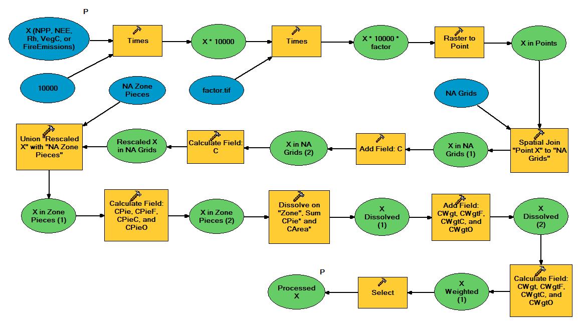
Figure 3. The aggregation model diagram within ArcGIS Model Builder
5.4. National GHG Inventories
The national GHG inventories database compiled for the NACP synthesis activities contains inventory-based data on productivity, ecosystem carbon stock change and harvested product stock change to produce estimates of land-atmosphere exchange of CO2 ( NEE) for the 2000 to 2006 time period for the Forest Lands and Crop Lands sectors in Canada and the United States. Additional information from national-level GHG inventories was used to fill in data on carbon balance in the Other Lands sector, including data on human and livestock consumption of harvested products. For Mexico, the national GHG inventories database accounts primarily for carbon flux caused by land use change according to the study by de Jong et al. (2010), which covers the period of 1993 to 2002. Data on carbon exchange for each sector are summarized according to GHG inventory “reporting zones.”
The methodology for producing estimates of NEE for each country/sector during the study period can be found from S4. Supporting Information Tables and Figures in Hayes et al. (2012). For additional information, please see the companion file, Regional-Standardized Inventory Zones.pdf, pp 14-15.
6. Data Access:
This data set is available through the Oak Ridge National Laboratory (ORNL) Distributed Active Archive Center (DAAC).
Data Archive:
Web Site: http://daac.ornl.gov
Contact for Data Center Access Information:
E-mail: uso@daac.ornl.gov
Telephone: +1 (865) 241-3952
7. References:
Bachelet, D., J.M. Lenihan, C. Daly, R.P. Neilson, D.S. Ojima, and W.J. Parton. 2001. MC1: A dynamic vegetation model for estimating the distribution of vegetation and associated ecosystem fluxes of carbon, nutrients, and water. USDA General Technical Report PNW-GTR-508. 95 pp. [http://www.treesearch.fs.fed.us/pubs/2923]
Bartholome, E., and A.S. Belward. 2005. GLC2000: a new approach to global land cover mapping from earth observation data. International Journal of Remote Sensing 26: 1959–1977. doi: 10.1080/01431160412331291297
de Jong, B., C. Anayab, O. Maserac, M. Olguína, F. Pazd, J. Etcheversd, R.D. Martínezc, G. Guerreroc, and C. Balbontíne. 2010. Greenhouse gas emissions between 1993 and 2002 from land-use change and forestry in Mexico. Forest Ecology and Management 260(10): 1689–1701. doi:10.1016/j.foreco.2010.08.011
Denning, A.S., et al. 2005. Science implementation strategy for the North American Carbon Program: A Report of the NACP Implementation Strategy Group of the U.S. Carbon Cycle Interagency Working Group. U.S. Carbon Cycle Science Program, Washington, DC. 68 pp.
Dickinson, R.E., K.W. Oleson, G. Bonan, F. Hoffman, P. Thornton, M. Vertenstein, et al. 2006. The Community Land Model and its climate statistics as a component of the Community Climate System Model. Journal of Climate 19(11): 2302-2324. doi:10.1175/JCLI3742.1
Environment Canada (2011) National Inventory Report 1990–2009: Greenhouse Gas Sources and Sinks in Canada. The Government of Canada’s Submission to the UN Framework Convention on Climate Change. Environment Canada, Ottawa, ON. Available at: http://www.ec.gc.ca/ges-ghg/(accessed 16 May 2011).
EPA (2011) Inventory of U.S. Greenhouse Gas Emissions and Sinks: 1990–2009. USEP-A #430-R-11-005. U.S. Environmental Protection Agency, Washington, DC. Avail-able at: http://www.epa.gov/climatechange/emissions/usinventoryreport.html (accessed 15 April 2011).
GLC2000. 2003. Global Land Cover 2000 database. European Commission, Joint Research Centre.
Hayes, D.J., D.P. Turner, G. Stinson, A.D. McGuire, Y. We1, T.O. West, L.S. Heath, B. de Jong, B.G. McConkey, R.A. Birdsey, W.A. Kurz, A.R. Jacobson, D.N. Huntzinger, Y. Pan, W.M. Post, and R.B. Cook. 2012. Reconciling estimates of the contemporary North American carbon balance among terrestrial biosphere models, atmospheric inversions, and a new approach for estimating net ecosystem exchange from inventory-based data. Global Change Biology 18(4): 1282–1299. doi:10.1111/j.1365-2486.2011.02627.x
Thornton, P.E., and N.A. Rosenbloom. 2005. Ecosystem model spin-up: estimating steady state conditions in a coupled terrestrial carbon and nitrogen cycle model. Ecological Modelling 189(1-2): 25-48. doi:10.1016/j.ecolmodel.2005.04.008
USDA Economic Research Service. 2010. Foreign Agricultural Trade of the United States (FATUS). [http://www.ers.usda.gov/data/fatus/]
USDA. 2008. U.S. Agriculture and Forestry Greenhouse Gas Inventory: 1990-2005, Technical Bulletin No. 1921, Global Change Program Office, Office of the Chief Economist, U.S. Department of Agriculture.
Y. Wei, W.M. Post, R.B. Cook, D.N. Huntzinger, P.E. Thornton, A. Jacobson, I. Baker, J. Chen, F. Chevallier, F. Hoffman, A. Jain, S. Liu, R. Lokupitiya, D.A. McGuire, A. Michalak, G.G. Moisen, R.P. Neilson, P. Peylin, C. Potter, B. Poulter, D. Price, J. Randerson, C. Rödenbeck, H. Tian, E. Tomelleri, G. van der Werf, N. Viovy, T.O. West, J. Xiao, N. Zeng, and M. Zhao. 2013. NACP Regional: Gridded 1-deg Observation Data and Biosphere and Inverse Model Outputs. Data set. Available on-line [http://daac.ornl.gov] from Oak Ridge National Laboratory Distributed Active Archive Center, Oak Ridge, Tennessee, U.S.A. http://dx.doi.org/10.3334/ORNLDAAC/1157
West, T., G. Marland, N. Singh, B. Bhaduri, and A. Roddy. 2009. The human carbon budget: an estimate of the spatial distribution of metabolic carbon consumption and release in the United States. Biogeochemistry 94: 29-41. doi:10.1007/s10533-009-9306-z
Wofsy, S.C., and R.C. Harriss. 2002. The North American Carbon Program (NACP). Report of the NACP Committee of the U.S. Interagency Carbon Cycle Science Program. U.S. Global Change Research Program, Washington, DC. 56 pp.
Additional Sources of Information:
Blackard, J.A. et. al. 2008. Mapping U.S. forest biomass using nationwide forest inventory data and moderate resolution information. Remote Sensing of the Environment. 112: 1658-1677. doi:10.1016/j.rse.2007.08.021
Chen, J.M., J. Liu, J. Cihlar, and M.L. Guolden. 1999. Daily canopy photosynthesis model through temporal and spatial scaling for remote sensing applications. Ecological Modelling 124: 99-119. doi:10.1016/S0304-3800(99)00156-8
Please also see the Reference section in the NACP Regional Synthesis - Description of Observations and Models document for publications related to the TBMs and IMs used in this study.