Documentation Revision Date: 2017-03-20
Data Set Version: V1
Summary
The atmospheric observations included (1) simulated remotely sensed column-averaged CO2 dry air mole fraction (denoted as XCO2) for the NASA Orbiting Carbon Observatory (OCO-2; Crisp et al., 2017) and (2) simulated tower-based flask sample CO2 concentrations. The land surface CO2 flux was estimated from (1) fossil fuel emissions (ffCO2) using the Vulcan fossil fuels emissions map and (2) the amount of CO2 added or removed by biosphere CO2 fluxes (bioCO2) as estimated with the CASA-GFED3 model. Contributions from fossil fuel and biosphere CO2 flux were calculated from simulated flask sample air measurements of radiocarbon in CO2 (Δ14C) following the work of Levin et al. (2003). The WRF-STILT model was applied to compute transport meteorology and region predictions.
The data files provide CO2 mixing ratio signals for November 2010 and May 2011, as derived for paired combinations of atmospheric observations and land surface fluxes. There are eight comma-separated (.csv) data files with this data set; four files for each month.
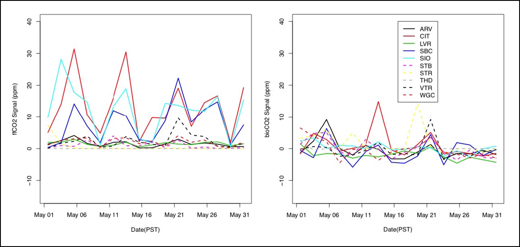
Figure 1. Predicted CO2 mixing ratio (ppm) signals for fossil fuel (left) and biosphere (right) exchanges for simulated flasks sampled for each tower site for month of May 2011. Negative biosphere exchange indicates carbon uptake by the land surface at some sites and sample dates in May, though some are positive, indicating that the contribution from respiration exceeds that from photosynthesis. Fossil emissions are always positive towards the atmosphere. From Fischer et al., 2017.
Citation
Fischer, M.L., N.C. Parazoo, K. Brophy, X. Cui, S. Jeong, J. Liu, R. Keeling, T.E. Taylor, K.R. Gurney, T. Oda, and H. Graven. 2017. CMS: CO2 Signals Estimated for Fossil Fuel Emissions and Biosphere Flux, California. ORNL DAAC, Oak Ridge, Tennessee, USA. http://dx.doi.org/10.3334/ORNLDAAC/1381
Table of Contents
- Data Set Overview
- Data Characteristics
- Application and Derivation
- Quality Assessment
- Data Acquisition, Materials, and Methods
- Data Access
- References
Data Set Overview
This study explored the potential for a prototype data collection and data analysis system to estimate regional and state-total fossil and bioCO2 exchanges in California using simulation experiments. The simulated atmospheric observations included remotely sensed column-averaged CO2 dry air mole fraction (denoted as XCO2) from the OCO-2 and tower-based observations of CO2 concentrations. The amount of CO2 added by fossil fuel emissions (ffCO2) and the amount of CO2 added or removed by biosphere CO2 fluxes (bioCO2) was calculated in flask air using measurements of radiocarbon in CO2 (Δ14C) following the work of Levin et al. (2003). The study aimed to distinguish between fossil fuel and biospheric influences from CO2 in flask samples.
Included with this data set are estimated CO2 mixing ratio signals due to carbon exchange from each of the 16 regions in California and a 17th region outside of the California but within the modeling domain during May, 2011 and November, 2010. The data were derived using a combination of the simulated data, the Vulcan fossil fuels emissions map and the CASA-GFED3 model.
The Vulcan 2.2 emissions map was used as the primary ffCO2 prior flux estimate and then uncertainties were estimated by comparing Vulcan with other ffCO2 emission data sets. Net biosphere CO2 fluxes were derived using the CASA-GFED3 model.
The WRF-STILT model was applied to compute transport meteorology and footprint predictions. A regionally specific inversion framework was used to solve for expected posterior uncertainties.
Project: Carbon Monitoring System (CMS)
The NASA Carbon Monitoring System (CMS) is designed to make significant contributions in characterizing, quantifying, understanding, and predicting the evolution of global carbon sources and sinks through improved monitoring of carbon stocks and fluxes. The System will use the full range of NASA satellite observations and modeling/analysis capabilities to establish the accuracy, quantitative uncertainties, and utility of products for supporting national and international policy, regulatory, and management activities. CMS will maintain a global emphasis while providing finer scale regional information, utilizing space-based and surface-based data and will rapidly initiate generation and distribution of products both for user evaluation and to inform near-term policy development and planning.
Related Publication:
Fischer, M.L., N. Parazoo, K. Brophy, X. Cui, S. Jeong, J. Liu, R. Keeling, T.E. Taylor, K. Gurney, T. Oda, and H. Graven. 2017. Simulating Estimation of California Fossil Fuel and Biosphere Carbon Dioxide Exchanges Combining In-situ Tower and Satellite Column Observations, J. Geophys. Res. Atmos., 122, doi:10.1002/2016JD025617
Data Characteristics
Spatial Coverage: Multiple points in California, USA
Spatial Resolution: 0.1 degree
Temporal Resolution: Hourly
Temporal Coverage: 20101101 to 20101129 and 20110501 to 20110531
Spatial Extent: (All latitude and longitude given in decimal degrees)
| Sites | Westernmost Longitude | Easternmost Longitude | Northernmost Latitude | Southernmost Latitude |
|---|---|---|---|---|
| California, USA | -124.151 | -115.963 | 42.82 | 32.20444 |
Data File Information
The data files provide CO2 signals for November 2010 and May 2011, as derived for paired combinations of atmospheric observations and land surface fluxes. There are four files for each month, for a total of eight comma-separated (.csv) data files with this data set.
Data are for the 16 regions (~air basins) in California and, the remaining land surface fluxes in the modeling domain outside California are represented as a 17th region.
Table 1. File names and descriptions.
| Biosphere flux data files | File description |
|---|---|
| (1) CASA_bioCO2_flask_region_201105.csv | Estimated CO2 signals from biosphere CO2 fluxes using the NASA-CASA model, and simulated flask data for May, 2011. |
| (2) CASA_bioCO2_flask_region_201011.csv | Estimated CO2 signals from biosphere CO2 fluxes using the NASA-CASA model, and simulated flask data for November, 2010. |
| (3) CASA_bioCO2_OCO2_region_201105.csv | Estimated CO2 signals from biosphere CO2 fluxes using the NASA-CASA model, and simulated OCO-2 data for May, 2011. |
| (4) CASA_bioCO2_OCO2_region_201011.csv | Estimated CO2 signals from biosphere CO2 fluxes using the NASA-CASA model, and simulated OCO-2 data for November, 2010. |
| Fossil fuel emissions data files | |
| (5) Vulcan_ffCO2_flask_region_201105.csv | Estimated CO2 signals using simulated flask data and the Vulcan 2.2 emissions map as the primary ffCO2 prior flux estimate for May, 2011. |
| (6) Vulcan_ffCO2_flask_region_201011.csv | Estimated CO2 signals using simulated flask data and the Vulcan 2.2 emissions map as the primary ffCO2 prior flux estimate for November, 2010. |
| (7) Vulcan_ffCO2_OCO2_region_201105.csv | Estimated CO2 signals using simulated OCO2 data and the Vulcan 2.2 emissions map as the primary ffCO2 prior flux estimate for May, 2011. |
| (8) Vulcan_ffCO2_OCO2_region_201011.csv | Estimated CO2 signals using simulated OCO2 data and the Vulcan 2.2 emissions map as the primary ffCO2 prior flux estimate for November, 2010. |
Table 2. Variables in the data files where CO2 signals were estimated using simulated OCO2 data (“OCO2” is in the file name).
| Column # | Column heading | Units/format | Description |
|---|---|---|---|
| 1 | site | text | Site= OCO2 (NASA Orbiting Carbon Observatory) |
| 2 | date | yyyymmdd | Date of predicted CO2 signal concentration measurement |
| 3 | longitude | decimal degrees | Longitude of simulated OCO2 orbit track and data retrieval |
| 4 | latitude | decimal degrees | Latitude of simulated OCO2 orbit track and data retrieval |
| 5-13 | reg01-reg17 | ppm | Estimated CO2 mixing ratio signals in parts per million at each of the 16 California regions and region 17 outside of California |
Table 3. Variables in the data files where CO2 signals were estimated using simulated flask data from 10 tower sites (“flask” is in the file name).
| Column # | Column heading | Units/format | Description |
|---|---|---|---|
| 1 | site | text | Site= 10 tower sites as shown in Table 4 |
| 2 | date | yyyymmdd | Date of estimated CO2 signal concentration measurement |
| 3 | longitude | decimal degrees | Longitude of the respective tower “site” as shown in Table 4 |
| 4 | latitude | decimal degrees | Latitude of the respective tower “site” as shown in Table 4 |
| 5-13 | reg01-reg17 | ppm | Estimated CO2 mixing ratio signals in parts per million at each of the 16 California regions and region 17 outside of California |
Application and Derivation
This study explored the potential for a prototype data collection and data analysis system to estimate regional and state-total fossil and bioCO2 exchanges in California using simulation experiments (Fischer et al., 2017).
These data could be useful for environmental air quality policy and climate change studies.
Quality Assessment
Contributions to uncertainties in predicted CO2 signals were estimated separately for the transport model, biosphere, and fossil fuel fluxes. Transport uncertainties were estimated by comparing predicted driving variables (e.g., winds and boundary layer depth) against observations at wind profiler and other sites in California. Biosphere flux uncertainties were predicted by propagating uncertainties in driving variables through the CASA model and by comparison with biosphere fluxes estimated in the Carbon Tracker model. Fossil fuel flux uncertainties were estimated by comparing variations for four fossil fuel models (Vulcan, EDGAR, FFDAS and ODIAC) in regionally summed emissions for 16 regions in California (Fischer et al., 2017).
The scaling factor Bayesian inversion method was used to quantify the effect of biases in flask and OCO-2 observations.
Data Acquisition, Materials, and Methods
Methods
This data set reports the results of a study that explored the potential for a prototype data collection and data analysis system to estimate regional and state-total fossil and biosphere CO2 (bioCO2) flux in California using simulated data and the CASA-GFED3 model (Fischer et al., 2017). The simulated atmospheric observations included remotely sensed column-averaged CO2 dry air mole fraction (denoted as XCO2) from OCO-2 and tower-based observations of CO2 concentrations, in conjunction with calculated radiocarbon in CO2 following the work of Levin et al. (2003). The study aimed to distinguish between fossil fuel and biospheric influences from CO2 in flask samples. The scaling factor Bayesian inversion method was used to quantify the effect of biases in flask and OCO-2 observations.
The data included with this data set provide predicted CO2 mixing ratio signals (ppm) from ffCO2 and bioCO2 flux in May 2011 and November 2010. Negative data exchange refers to carbon uptake by the land surface at some sites and sample dates in May, though some are positive, indicating that the contribution from respiration exceeds that from photosynthesis. In November, bioCO2 signals are generally positive because respiratory fluxes dominate.
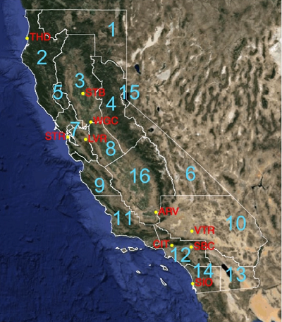
Figure 2. Study area in California showing the 16 air basin regions and 10 tower sites. Region 17 is the area outside of California.
Simulated data
Flask samples: The ground-based measurements were simulated from 10 existing air sampling sites located in major urban and selected rural areas across California (Table 4). It was assumed that flask samples would be collected every two days at 2200 GMT (1400 PST) at each site over two example months when net biosphere exchange of CO2 is expected to be positive (November 2010) and negative (May 2011) (Fischer et al., 2017).
Table 4. Tower measurement sites in California.
| Site Location | Location | Latitude | Longitude | Inlet Height (m, a.g.l.) |
|---|---|---|---|---|
| ARV | Arvin | 35.24 | -118.79 | 10 |
| CIT | Caltech, Pasadena | 34.14 | -118.12 | 10 |
| LVR | Livermore | 37.67 | -121.71 | 27 |
| SBC | San Bernardino | 34.09 | -117.31 | 58 |
| SIO | Scripps | 32.87 | -117.26 | 10 |
| STB | Sutter Buttes | 39.21 | -121.82 | 10 |
| STR | San Francisco | 37.76 | -122.45 | 232 |
| THD | Trinidad Head | 41.05 | -124.15 | 20 |
| VTR | Victorville | 34.61 | -117.29 | 90 |
| WGC | Walnut Grove | 38.27 | -121.49 | 91 |
OCO-2: For the time period analyzed, which was prior to the acquisition of real OCO-2 observations (Crisp et al., 2017), synthetic OCO-2 soundings were generated using the OCO-2 simulator at Colorado State University (O’Brien, 2009). These simulations were based on mission specifications in 2012 of collecting only four footprints per measurement frame. However, prior to launch, mission status doubled this to retrieve the full eight footprints per frame. The simulations included clouds and aerosols taken from a database of Cloud-Aerosol Lidar and Infrared Pathfinder Satellite Observations (CALIPSO) profile data, and were screened using a total optical depth (TOD) threshold of 0.3. Simulations were run over a 32-day period in September and October to account for 16-day repeat cycles for nadir and glint viewing modes. Similar orbit tracks and data yield were assumed for inversion simulation experiments in November 2010 and May 2011, although in reality, cloud coverage and glint orbits will shift during the year (Fischer et al., 2017).
CASA-GFED3: Net biosphere CO2 fluxes were derived using the CASA-GFED3 model with 0.5 x 0.5-degree resolution adapted for the NASA CMS Flux Pilot Project. The model employs remotely sensed meteorology together with vegetation index from MODIS and an estimated light use efficiency parameterization to simulate net primary productivity, and a soil model to simulate heterotrophic respiration and thereby, net ecosystem production. In this implementation, the diurnal cycle from the 1.25 x 1.0-degree fluxes was imposed onto the nearest neighbor 0.5 x 0.5-degree monthly mean fluxes to approximate hourly resolved biosphere fluxes at 0.5-degree resolution.
Vulcan 2.2 emissions map: In order to characterize the likely spatial and temporal variations of ffCO2 emissions across California, the Vulcan 2.2 emissions map was used as the primary ffCO2 prior flux estimate. Vulcan provides hourly resolved fossil fuel CO2 emissions on a 0.1 x 0.1-degree gridded product of emissions grid for 2002 that takes into account weekday and weekend variations in emissions from the location of power plants, roads, and industrial facilities including cement production. Even though the focus was on the years 2010-11, the Vulcan 2.2 product for the year 2002 was used without modification. The EDGAR (version FT2010, EDGAR, 2011) 0.1 x 0.1-degree time-invariant emissions map was used as an alternate ffCO2 prior flux estimate.
Atmospheric Transport and CO2 Signal Prediction
The WRF-STILT model (Lin et al., 2003) was applied to compute transport meteorology and footprint predictions for May 2011 and November 2010. WRF version 3.5.1 was used to simulate meteorology in domains covering western North America at 36 and 12 km, nesting down over sub-regions of California at 4 and 1.3-km resolutions following work described in Jeong et al. (2013). The five-layer thermal diffusion land surface model was used for May when irrigation provides an additional source of land surface moisture in California, and the NOAH land surface model was used for November. To compute CO2 measurement sensitivity to surface fluxes (footprints) from hourly WRF outputs, an ensemble of 500 STILT particles were released from each receptor and run backwards in time for seven days driven with meteorology from WRF output. In the case of OCO-2 receptors, 500 particles were released along nadir vertical columns and distributed across 10 vertical layers of 1-km thickness from the land surface to the top layer of the WRF model atmosphere of 10 km altitude, corresponding to ~ 75% of the atmospheric column. The density of particles per layer varies in proportion to the mean layer pressure along the column to approximate the column profile. While this approach does not include a more detailed representation of the OCO-2 observation profile, it is unlikely to strongly affect the results.
In general, footprint sensitivity is largest near the receptor sites and tracks the upwind direction backward in time. For each site and time point, the simulated hourly resolved CO2 signals were calculated by summing over the footprint times the corresponding flux over each of the 16 regions within California, and remaining land surface fluxes in the modeling domain outside California for a 17th region. CO2 signals refer to the local enhancement or depletion in CO2 concentration caused by fossil fuel emissions or biospheric exchange occurring within the domain.
Data Access
These data are available through the Oak Ridge National Laboratory (ORNL) Distributed Active Archive Center (DAAC).
CMS: CO2 Signals Estimated for Fossil Fuel Emissions and Biosphere Flux, California
Contact for Data Center Access Information:
- E-mail: uso@daac.ornl.gov
- Telephone: +1 (865) 241-3952
References
Crisp, D., Pollock, H. R., Rosenberg, R., Chapsky, L., Lee, R. A. M., Oyafuso, F. A., Frankenberg, C., O'Dell, C. W., Bruegge, C. J., Doran, G. B., Eldering, A., Fisher, B. M., Fu, D., Gunson, M. R., Mandrake, L., Osterman, G. B., Schwandner, F. M., Sun, K., Taylor, T. E., Wennberg, P. O., and Wunch, D. (2017), The on-orbit performance of the Orbiting Carbon Observatory-2 (OCO-2) instrument and its radiometrically calibrated products, Atmos. Meas. Tech., 10, 59-81, DOI:10.5194/amt-10-59-201
Fischer, M.L., N. Parazoo, K. Brophy, X. Cui, S. Jeong, J. Liu, R. Keeling, T.E. Taylor, K. Gurney, T. Oda, and H. Graven. 2017. Simulating Estimation of California Fossil Fuel and Biosphere Carbon Dioxide Exchanges Combining In-situ Tower and Satellite Column Observations, J. Geophys. Res. Atmos., 122, doi:10.1002/2016JD025617.
Jeong, S., Y-K. Hsu, A.E. Andrews, L. Bianco, P. Vaca, J.M. Wilczak, and M.L. Fishcer. (2013). A multitower measurement network estimate of California's methane emissions. Journal of Geophysical Research: Atmospheres 118(19): 2013JD019820. DOI: 10.1002/jgrd.50854
Levin, I., B. Kromer, M. Schmidt and H. Sartorius (2003). A novel approach for independent budgeting of fossil fuel CO2 over Europe by 14CO2 observations. Geophysical Research Letters, 30. DOI: 10.1029/2003GL018477
Lin, J. C., et al. (2003), A near-field tool for simulating the upstream influence of atmospheric observations: The Stochastic Time-Inverted Lagrangian Transport (STILT) model, Journal of Geophysical Research-Atmospheres, 108 (D16) DOI: 10.1029/2002JD003161
O’Brien, D. M., Polonsky, I., O’Dell, C., and Carheden, A. 2009. Orbiting Carbon Observatory (OCO), Algorithm Theoretical Basis Document: The OCO simulator, Technical Report ISSN 0737-5352-85, 2009, Cooperative Institute for Research in the Atmosphere, Colorado State University (ftp://ftp.cira.colostate.edu/ftp/TTaylor/publications/20090813_OCO_simulator.pdf).