Documentation Revision Date: 2018-04-16
Data Set Version: 1
Summary
ACES is the first multi-state regional bottom-up inventory to report hourly FFCO2 fluxes at a 1 x 1 km gridded resolution for all major carbon-emitting sectors, using an extensive database of high-resolution spatial proxies.
There are 30 data files with this dataset; 12 files with the annual 2011 data (total and by sector) in GeoTIFF (.tif) format and 18 files with the hourly 2013 and 2014 data (total and by sector for each year) in netCDF (.nc4) format.
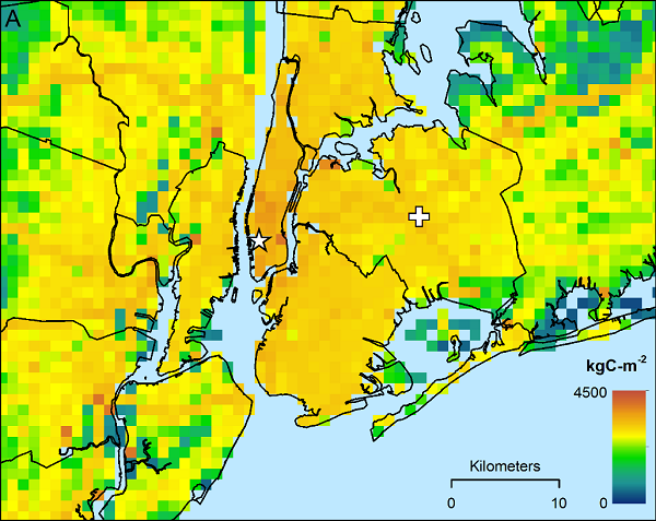
Figure 1. Shown are ACES total 2011 annual FFCO2 emissions for the New York City metropolitan area. Highlighted are a mixed residential and commercial zone in downtown Manhattan (white star) and a residential neighborhood in Forest Hills, Queens (white cross). The investigation of the hourly inventory revealed that the diurnal pattern of vehicle traffic dominates the signal in Queens, while in Manhattan the hourly fluxes are driven by the influence of daily meteorology on building heating demand. (from Gately and Hutyra, 2017).
Citation
Gately, C., and L.R. Hutyra. 2018. CMS: CO2 Emissions from Fossil Fuels Combustion, ACES Inventory for Northeastern USA. ORNL DAAC, Oak Ridge, Tennessee, USA. https://doi.org/10.3334/ORNLDAAC/1501
Table of Contents
- Data Set Overview
- Data Characteristics
- Application and Derivation
- Quality Assessment
- Data Acquisition, Materials, and Methods
- Data Access
- References
- Data Set Revisions
Data Set Overview
This dataset provides estimates of annual and hourly carbon dioxide (CO2) emissions from the combustion of fossil fuels (FF) for 13 states across the Northeastern United States. The Anthropogenic Carbon Emissions System (ACES) was used to estimate annual FFCO2 emissions for nine different emissions source sectors on a 1 x 1 km spatial grid, for the year 2011. Hourly estimates of FFCO2 for the years 2013 and 2014 were derived from the 2011 annual emissions by holding the total emissions constant, but accounting for seasonal and daily variations in meteorology, fuel consumption, and traffic patterns across these two years.
ACES is a bottom-up approach providing the first multi-state regional inventory to report hourly FFCO2 fluxes at a 1 x 1 km gridded resolution for all major carbon-emitting sectors, using an extensive database of high-resolution spatial proxies.
Project: Carbon Monitoring System
The NASA Carbon Monitoring System (CMS) is designed to make significant contributions in characterizing, quantifying, understanding, and predicting the evolution of global carbon sources and sinks through improved monitoring of carbon stocks and fluxes. The System will use the full range of NASA satellite observations and modeling/analysis capabilities to establish the accuracy, quantitative uncertainties, and utility of products for supporting national and international policy, regulatory, and management activities. CMS will maintain a global emphasis while providing finer scale regional information, utilizing space-based and surface-based data and will rapidly initiate generation and distribution of products both for user evaluation and to inform near-term policy development and planning.
Related Publication:
Gately, C. K., & Hutyra, L. R. (2017). Large uncertainties in urban-scale carbon emissions. Journal of Geophysical Research: Atmospheres, 122, 11,242–11,260. https://doi.org/10.1002/2017JD027359
Related Data Set:
Gately, C.K., L.R. Hutyra, and I.S. Wing. 2015. CMS: DARTE Annual On-road CO2 Emissions on a 1-km Grid, Conterminous USA, 1980-2012. ORNL DAAC, Oak Ridge, Tennessee, USA. http://dx.doi.org/10.3334/ORNLDAAC/1285
Acknowledgements
This research was supported primarily by the National Aeronautics and Space Administration Carbon Monitoring System program (grant NNH13CK02C and NNX16AP23G) with additional support from the National Oceanic and Atmospheric Administration (NOAA #NA14OAR4310179). We thank Jackie Getson for technical assistance in the creation of this inventory, along with Andrew Trlica. We are also grateful for useful discussions and feedback from Kevin Gurney, Ian Sue Wing, and Andrew Reinmann.
Data Characteristics
Spatial Coverage: The Northeast US
Spatial Resolution: 1-km grid
Temporal Coverage: Data cover the years 2011 and 2013-2014
Temporal Resolution: Annual and hourly
Study Area (All latitudes and longitudes are given in decimal degrees)
| Site | Westernmost Longitude | Easternmost Longitude | Northernmost Latitude | Southernmost Latitude |
|---|---|---|---|---|
| Northeastern US | -81.7794 | -65.9319 | 49.19362 | 34.51113 |
Data File Information
There are 30 data files with this dataset; 12 files with the annual 2011 data (total and by sector) in GeoTIFF (.tif) format and 18 files with the hourly 2013 and 2014 data (total and by sector for each year) in netCDF (.nc4) format.
The data reported are emissions of FFCO2 from the residential, commercial, industrial, on-road, non-road mobile, marine, oil and gas, and rail sectors, and point sources, which includes electric power generation, industrial facilities, and aircraft take-off and landing operations.
Important Data User Note:
Please note that the units for the GeoTIFF format files are as Carbon (kg C km-2 y-1) and the units for the the NetCDF format files are as CO2 (kg CO2 km-2 h-1).
2011 Annual Data in GeoTIFF Format:
Table 1. File names and descriptions.
| File Name | Description |
|---|---|
| ACES_kgC_2011_TOTAL.tif | Total CO2 emissions (kg C km-2 y-1) from all sources and sectors |
| ACES_kgC_2011_RAIL.tif | CO2 emissions (kg C km-2 y-1) from the rail sector obtained from NEI and converted to CO2 using emission factors from EPA (2009a) |
| ACES_kgC_2011_COM.tif | CO2 emissions (kg C km-2 y-1) from the commercial sector |
| ACES_kgC_2011_OILGAS.tif | CO2 emissions (kg C km-2 y-1) associated with oil and gas production at the county level |
| ACES_kgC_2011_POINT_ELEC.tif | CO2 emissions (kg C km-2 y-1) from point sources from electricity generating facilities |
| ACES_kgC_2011_AIR.tif | CO2 emissions(kg C km-2 y-1) from the aircraft sector estimated for near-surface emissions only, covering aircraft taxiing, take-off and landing operations, and other ground-based airport vehicles and on-site stationary combustion sources |
| ACES_kgC_2011_NONROAD.tif | CO2 emissions (kg C km-2 y-1) from vehicles that are not operating on the public road network (e.g. construction vehicles, agricultural vehicles, lawn and garden equipment) |
| ACES_kgC_2011_RES.tif | CO2 emissions (kg C km-2 y-1) from the residential sector |
| ACES_kgC_2011_NONPOINT_IND.tif | CO2 emissions (kg C km-2 y-1) from nonpoint sources in the industrial sector |
| ACES_kgC_2011_MARINE.tif | CO2 emissions (kg C km-2 y-1) from the marine sector converted to CO2 using emissions factors from EPA (2009b) and assigned to waterways and port area |
| ACES_kgC_2011_ONROAD.tif | CO2 emissions (kg C km-2 y-1) based on annual road-level CO2 emissions estimates reported by the Database of Road Transportation Emissions (DARTE) (Gately et al., 2015) |
| ACES_kgC_2011_POINT_NONELEC.tif | CO2 emissions (kg C km-2 y-1) from point sources from non-electricity generating facilities |
Table 2. Properties of the GeoTIFF files.
| Filename | Number of Bands | Range of Values | Fill Value | Data Type |
|---|---|---|---|---|
| ACES_kgC_2011_TOTAL.tif | 1 | 0 - 4.42E+09 | -9999 | Float 64 |
| ACES_kgC_2011_RAIL.tif | 1 | 0 - 1 | -9999 | Float 64 |
| ACES_kgC_2011_COM.tif | 1 | 0 - 1.75E+08 | -9999 | Float 64 |
| ACES_kgC_2011_OILGAS.tif | 1 | 0 - 8518277 | -9999 | Float 64 |
| ACES_kgC_2011_POINT_ELEC.tif | 1 | 0 - 4.42E+09 | -9999 | Float 64 |
| ACES_kgC_2011_AIR.tif | 1 | 0 - 20570304 | -9999 | Float 64 |
| ACES_kgC_2011_NONROAD.tif | 1 | 0 - 4817478 | -9999 | Float 64 |
| ACES_kgC_2011_RES.tif | 1 | 0 - 27346016 | -9999 | Float 64 |
| ACES_kgC_2011_NONPOINT_IND.tif | 1 | 0 - 3530807 | -9999 | Float 64 |
| ACES_kgC_2011_MARINE.tif | 1 | 0 - 38.9 | -9999 | Float 64 |
| ACES_kgC_2011_ONROAD.tif | 1 | 0 - 1.02E+08 | -9999 | Float 64 |
| ACES_kgC_2011_POINT_NONELEC.tif | 1 | 0 - 1.06E+09 | -9999 | Float 64 |
2013 and 2014 Hourly Data in NetCDF Format:
Table 3. File names and descriptions. XXXX in the file name is the year: either 2013 or 2014.
| File Name | Description |
|---|---|
| total_hourly_CO2_flux_XXXX.nc4 | Total hourly CO2 (kg CO2 km-2 h-1) emissions from all sectors |
| res_hourly_CO2_flux_XXXX.nc4 | Hourly CO2 (kg CO2 km-2 h-1) emissions from the residential sector |
| onroad_hourly_CO2_flux_XXXX.nc4 | Hourly CO2 (kg CO2 km-2 h-1) emissions associated from on-road sources |
| oilgas_hourly_CO2_flux_XXXX.nc4 | Hourly CO2 (kg CO2 km-2 h-1) emissions from the oil and gas production sector |
| offroad_hourly_CO2_flux_XXXX.nc4 | Hourly CO2 (kg CO2 km-2 h-1) emissions from vehicles that are not operating on the public road network (e.g. construction vehicles, agricultural vehicles, lawn and garden equipment) |
| nonelec_hourly_CO2_flux_XXXX.nc4 | Hourly CO2 (kg CO2 km-2 h-1) emissions from non-electricity generating facilities |
| elec_hourly_CO2_flux_XXXX.nc4 | Hourly CO2 (kg CO2 km-2 h-1) emissions from electricity generating facilities |
| airport_hourly_CO2_flux_XXXX.nc4 | Hourly CO2 (kg CO2 km-2 h-1) emissions from the aircraft sector estimated for near-surface emissions only, covering aircraft taxiing, take-off and landing operations, and other ground-based airport vehicles and on-site stationary combustion sources |
| indcom_hourly_CO2_flux_XXXX.nc4 | Hourly CO2 (kg CO2 km-2 h-1) emissions from the industrial and commercial sectors |
Table 4. Variables in all NetCDF files. The variables below are in all 2013 and 2014 hourly .nc4 files.
| Variable | Units/format | Description |
|---|---|---|
| flux_CO2 | kg CO2 km-2 h-1 | Hourly surface upward mass flux of CO2 (kg CO2 km-2 h-1) |
| lat | decimal degrees | Degrees north |
| lon | decimal degrees | Degrees east |
| time | hours since 2013-01-01 00:00:00 | Middle of each hour |
| time_bnds | hours since 2013-01-01 00:00:00 | Start and end time for each time stamp |
| x | m | Projection x coordinate |
| y | m | Projection y coordinate |
Table 5. Spatial extents of all data files.
| Files | North_lat | South_lat | East_long | West_long |
|---|---|---|---|---|
| NetCDF-hourly data files | 49.19362 | 34.51113 | -65.9327 | -81.7687 |
| GeoTIFF files | 49.18639 | 34.50833 | -65.9319 | -81.7794 |
Application and Derivation
The ACES methodology is designed for easy updating, making it suitable for emissions monitoring under most city, regional, and state greenhouse gas mitigation initiatives, in particular for the small and medium-sized cities that lack the resources to regularly perform their own bottom-up emissions inventories.
These data could be useful to climate change studies and policies regarding fossil fuel combustion.
Quality Assessment
A comparison of ACES with three of the most commonly used global FFCO2 inventories shows that even at broad regional scales the overall uncertainty in emissions estimates is as high as 20%. While the ACES inventory itself has a relatively modest total uncertainty of ~8.6%, the overall disagreement between ACES and the major global inventories implies that this uncertainty may be somewhat larger. Two inventories constructed from the same data sources (i.e. ODIAC and FFDAS) report different regional emissions totals (Δ12%) for our domain, emphasizing how minor differences in included source sectors and the downscaling algorithms can produce significant differences at sub-national scales (Gately and Hutyra, 2017).
Data Acquisition, Materials, and Methods
The Anthropogenic Carbon Emissions System (ACES) is a bottom-up high-resolution model for FFCO2. ACES was used to estimate CO2 annual emissions resulting from the combustion of fossil fuels for the year 2011, on a 1 x 1 km spatial grid, partitioned by emitting sector. The 2011 annual emissions were then used to calculate hourly emissions for 2013 and 2014 holding the total emissions constant, but accounting for seasonal and daily variations in meteorology, fuel consumption, and traffic patterns across these two years (Gately and Hutyra, 2017).
Data Sources
Emissions of FFCO2 from the residential, commercial, industrial, non-road mobile, marine, and rail sectors were derived from the U.S. Environmental Protection Agency’s (EPA) National Emissions Inventory (NEI) for 2011 (EPA, 2014a). Emissions from point sources, which include electric power generation, industrial facilities, and aircraft take-off and landing operations, were estimated using a combination of data from the NEI and from the EPA Greenhouse Gas Reporting Program (GHGRP) (EPA, 2014b). On-road CO2 emissions were obtained from the Database of Road Transportation Emissions (DARTE) (Gately et al., 2015).
The NEI reports annual emissions of carbon monoxide (CO) at the county scale for most of the non-point sources (residential, commercial, some industrial, non-road vehicles, and railway). Marine CO emissions in NEI are reported for port areas, and inland and near-coastal waterways. For point sources, NEI and GHGRP report annual CO and CO2 emissions, respectively, for each facility, with an accompanying latitude and longitude. Emissions factors from the EPA WEBFire database (EPA , 2014c) and from Gurney et al. (2010) were used to convert CO estimates to CO2, depending on fuel type and combustion process. County-level CO2 emissions were then spatially downscaled using spatial proxies specific to each source sector (Gately and Hutyra, 2017).
Data on oil and gas wellhead locations were obtained from multiple state sources (New York State DEP, 2016; Pennsylvania DEP, 2016; Virginia Dept. of Mines, Minerals, and Energy, 2016; West Virginia DEP, 2016) and used to assign emissions to individual wellheads within each county.
Table 6. Data sources used to derive the emissions inventories. A bibliography for the sources is provided at the end of this section.
| Sector | Data Source | Native Spatial Resolution |
|---|---|---|
| Residential | NEI | County |
| Commercial | NEI | County |
| Industrial | NEI GHGRP | County/point |
| Electricity | NEI GHGRP | Point |
| Airport | NEI | Point |
| On-road | DARTE | Line |
| Off-road | NEI | County |
| Oil and Gas | EPA | County/Point |
| Marine | NEI | Area |
| Railroad | NEI | Line |
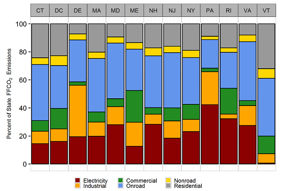
Figure 2. State-level emissions shares by source sector from ACES. Oil and gas production sector emissions are included in the industrial sector (Figure S2, Gately and Hutyra, 2017) .
Methods
Aircraft sector
Aircraft sector emissions were estimated for near-surface emissions only, covering aircraft taxiing, take-off and landing operations, and other ground-based airport vehicles and on-site stationary combustion sources. All emissions for this sector were treated as point sources located at the airport location reported by the NEI.
Data were downscaled from annual to daily using FAA - ATADS data on daily takeoffs and landings at each airport in domain. Hourly factors were obtained from a sample of weekday and weekend flight data obtained from the public version of www.flightstats.com .
Rail Sector
Railway CO emissions were obtained from NEI and converted to CO2 using emission factors from EPA (2009a). Emissions were summed by county and then spatially distributed onto the NEI-provided “Rail Line Shape Files” GIS layer using the “2011NEIv2 Shape Fractions of County Emissions for Rail and Commercial Marine”, both available at http://www.epa.gov/ttnchie1/net/2011inventory.html.
No downscaling; railway emissions were given a flat hourly time structure, as no data on seasonal, monthly or diurnal patterns in activity was available.
Marine Sector
Emissions were summed by county and then spatially distributed onto the NEI-provided “Rail Line Shape Files” GIS layer using the “2011NEIv2 Shape Fractions of County Emissions for Rail and Commercial Marine”, both available at http://www.epa.gov/ttnchie1/net/2011inventory.html. Marine vessel CO emissions were converted to CO2 using emissions factors from EPA (2009b) and assigned to waterways and port areas using the shapefile above.
All marine vessels that burn residual oil as fuel were assumed to have the emissions characteristics of ‘Ocean-Going Vessels’ and are all 'Medium-Speed Diesel'. Marine vessels that burn ‘Diesel Fuel’ in the NEI 'Port Emissions' category were assumed to be 50% ‘Ocean-Going Vessels’ and 50% ‘Harbor Craft’. Marine vessels that burn diesel fuel in the 'Underway emissions' category were assumed to be 100% ‘Harbor Craft’. Harbor Craft activity were partitioned (both in port and underway) as 25% Category 2 vessels and 75% Category 1 vessels, following EPA (2008). For Category 1 Harbor Craft, a CO emission factor of 1.5 g / kWh was used which is the median value for Tier 0 / Tier 1 / Category 1 vessels. A CO emission factor of 1.1 was used for Category 2 Harbor Craft. It was assumed that there are no Tier 2 craft. The CO2 emission factor for all Harbor Craft is 690 g/kWh, as in Table 3.8 of EPA (2008).
No downscaling; marine emissions are given a flat hourly time structure, as no data on seasonal, monthly or diurnal patterns in activity was available.
Electricity-generation Facilities and Non-electricity Generation Facilities
The NEI point file and GHGRP point file were partitioned into electricity-generation facilities and non-electricity generation facilities. Airport emissions from airplane taxiing, takeoff, and landing were removed and used to generate the airport sector emissions. Railroad equipment was also excluded. CO2 emissions from point sources were incorporated that report under the Greenhouse Gas Reporting Program, as these emissions are directly reported by each facility as CO2, which reduces the potential errors associated with using CO / CO2 conversion factors as was done for the NEI point source facilities.
For the 14,883 NEI point sources, CO emissions were converted into CO2 emissions using emissions factors from EPA (2014c) and from Gurney et al. 2010. The GHGRP reports emissions from each facility as CO2, which reduces the uncertainty associated with conversion factors. Where possible we use the GHGRP emissions (N=1,016). Annual, county-level CO emissions for non-point industrial sources were obtained from the NEI for industrial sources that are too small to be included in the NEI Point source or GHGRP databases.
Data were downscaled from annual to hourly emissions using hourly energy consumption by power stations reported to EPA continuous air quality monitoring division (CAMD). Annual emissions were assigned an hourly factor based on nearest CAMD power station. Hourly factor = each hour's share of annual total energy consumption.
Residential and Commercial Building Sector
Annual CO emissions from NEI at the county scale were used for the residential and commercial building sectors. Emissions were summarized into five categories: Fuel Oil, Gas, LPG, Wood, and Coal. CO was converted to to CO2 using emissions factors from the EPA WEBFire database (EPA, 2014c) and from Gurney et al. (2010) depending on fuel type and combustion process.
Commercial emissions were downscaled from county to Census Block using the number of jobs in each Block obtained from the Longitudinal Employment-Household Dynamics database (LODES) (U.S. Census Bureau, 2014). LODES was not available for Massachusetts, therefore the Massachusetts Tax Assessor Parcel data (Metropolitan Area Planning Council, 2014) was used to assign emissions based on the building square footage within each commercial-use parcels. For the LODES data, the number of jobs in each Census Block was divided by the total jobs in the county to produce an allocation factor. County total emissions were then multiplied by the factor for each Block to produce Block total emissions estimates.
Residential emissions were downscaled from county scale to Census Block Groups, using data on the number of households in each Census Block Group partitioned by type of home heating fuel (U.S. Census Bureau, 2015).
Industrial
Non-point industrial emissions were left at the county scale; point emissions were left at the native scale.
The downscaling method was according to the commercial sector above.
Oil and Gas Sector
CO2 emissions associated with oil and gas production at the county level were calculated using the EPA Oil and Gas Emission Estimation tool (http://www.epa.gov/ttnchie1/net/2011inventory.html). Data on oil and gas wellhead locations were obtained from multiple state sources and used to assign emissions to individual (point) wellheads within each county. The tool partitions emissions into four well-type categories: Oil, Gas, Combined Oil & Gas, and Water. County emissions were evenly distributed across all wells in a county by activity status and well type. Well location data was unavailable for Maryland, so emissions were distributed evenly across each county. Water injection-related emissions were distributed evenly to all wells in each county. If the well location data included a “combined” type the wells were assigned the “combined” emissions, otherwise the emissions were distributed evenly across the other well types. Other well types, if provided, (e.g. geothermal) were excluded from the emission allocation; only oil, gas, and combined oil and gas wells were assigned an emissions value. If there were oil emissions reported in NEI but no oil wells reported in the county, the emissions were averaged across the gas wells in that county (or vice versa). West Virginia did not have well type available; emissions were averaged evenly across all wells. A uniform time structure was used for emissions from this sector.
The oil and gas data are the same for both years. and there was no downscaling of the data. The time slices are all identical as there was no data to disaggregate annual emissions into hourly emissions. Therefore the data was distributed evenly across every hour of the year. Each hourly value was equal to the annual value divided by 8760.
Non-road Vehicles
For emissions from vehicles that are not operating on the public road network (e.g. construction vehicles, agricultural vehicles, lawn and garden equipment), estimates of county-level CO2 were obtained from the NONROAD2008 model included in the EPA MOVES2014a (Motor Vehicle Emission Simulator) model, available at https://www.epa.gov/moves/nonroad-model-nonroad-engines-equipment-and-vehicles. NONROAD2008 provides time-varying emissions estimates by month and by weekday / weekend, however this time structure was developed based on data from the NONROAD2005 model, and has not been updated since then. This is the same time structure used in the Vulcan Project ‘nonroad’ emissions layer, as Vulcan estimated emissions using the NONROAD2005 model (Gurney et al. 2010). The temporal structure of the Vulcan 2002 ‘nonroad’ layer was applied to the 2011 annual CO2 estimates to produce both the 2013 and 2014 hourly estimates.
Non-road emissions were given a uniform spatial distribution within each county, as no data on within-county spatial patterns was available. Due to data paucity, no uncertainty estimates were made for this sector.
On-road Sector
ACES onroad emissions are based on annual road-level CO2 emissions estimates reported by the Database of Road Transportation Emissions (DARTE) (Gately et al,. 2015). The magnitude uncertainty in DARTE emissions was calculated following the methods used in Gately et al. (2013) and Mendoza et al. (2013). One-sigma uncertainties in the levels of vehicle miles travelled (VMT) reported by the Federal Highway Administration (2017) were used and then propagated through the DARTE emissions model. Annual CO2 emissions were then downscaled to hourly estimates using hourly vehicle counts obtained from 492 in-road automatic traffic recorders (ATRs) spread across Connecticut, Maryland, Massachusetts, New Hampshire, New York, Pennsylvania, Vermont and Virginia. Each hourly share of annual total traffic was used to assign emissions to each hour. Each 1-km grid cell was assigned the hourly shares from nearest ATR station.
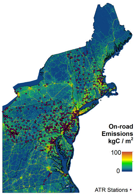
Figure 3. Map of Automatic Traffic Recorder (ATR) station locations used to temporally downscale DARTE annual FFCO2 emissions from the on-road sector to hourly ACES emissions. Each ATR shown provides hourly traffic counts for a full year. Each ACES grid cell was assigned the temporal pattern of the nearest ATR station. Background shows annual total emissions in ACES for the on-road sector in 2011 (Figure S5, Gately and Hutyra, 2017).
Table 7. Bibliography for data sources as cited above.
| Data Source Bibliography |
|---|
|
Data Access
These data are available through the Oak Ridge National Laboratory (ORNL) Distributed Active Archive Center (DAAC).
CMS: CO2 Emissions from Fossil Fuels Combustion, ACES Inventory for Northeastern USA
Contact for Data Center Access Information:
- E-mail: uso@daac.ornl.gov
- Telephone: +1 (865) 241-3952
References
Gately, C. K., & Hutyra, L. R. (2017). Large uncertainties in urban-scale carbon emissions. Journal of Geophysical Research: Atmospheres, 122, 11,242–11,260. https://doi.org/10.1002/2017JD027359
Gately, C. K., L.R. Hutyra, and I. Sue Wing. 2015. Cities, Traffic, and CO2: A Multidecadal Assessment of Trends, Drivers, and Scaling Relationships. Proc. Natl. Acad. Sci. 112 (16), 4999–5004.
Gately, C.K., L.R. Hutyra, I. Sue Wing, and M.N. Brondfield. 2013. A Bottom up Approach to on-Road CO 2 Emissions Estimates: Improved Spatial Accuracy and Applications for Regional Planning. Environ. Sci. Technol. 47 (5), 2423–2430.
Gurney, K.R., D. Mendoza, Y. Zhou, M. Fisher, C. Miller, S. Geethakumar, and S. De La Rue Dy Can. 2010. Vulcan Science Methods Documentation, Version 2.0. Available at: http://vulcan.project.asu.edu/pdf/Vulcan.documentation.v2.0.online.pdf, (Accessed on September 1, 2015).
Mendoza, D., K. R. Gurney, S. Geethakumar, V. Chandrasekaran, Y. Zhou, Y, and I. Razlivanov. 2013. Implications of uncertainty on regional CO2 mitigation policies for the U.S. onroad sector based on a high-resolution emissions estimate. Energy Policy, 55, 386–395. http://doi.org/10.1016/j.enpol.2012.12.027
Data Set Revisions
This dataset was revised on April 16, 2018, with the following changes:
- units in the netCDF data files were changed from Carbon Flux (kg C km-2 y-1) to specifically CO2 Flux (kg CO2 km-2 h-1)
- time units have been corrected to indicate standard UTC time
- The file ACES_kgC_2011_ONROAD.tif was replaced with corrected values