Documentation Revision Date: 2016-09-13
Data Set Version: V1
Summary
The fifteen MsTMIP models included: BIOME_BGC, CLM, CLM4VIC, CLASS_CTEM, DLEM, GTEC, ISAM, LPJ, ORCHIDEE, SIB3, SIBCASA, TEM6, TRIPLEX-GHG, VEGAS, and VISIT. Additionally, four ensemble products were included: un-weighted (naive) ensemble mean, un-weighted (naive) ensemble standard deviation, weighted (optimal) ensemble mean, and weighted (optimal) ensemble standard deviation.
There are 670 files in NetCDF v4 format with this data set. This includes a separate file for each product (15 models and four ensemble products) per year for seven years, plus five land area files.
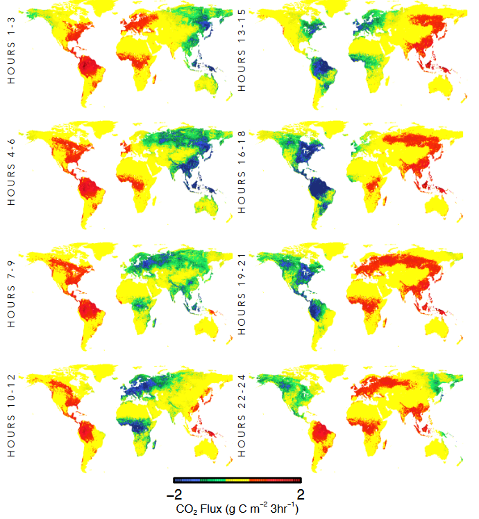
Figure 1. Vegetation productivity (blues/greens) follows the sun for a day. NEE for 3-hourly periods on July 1, 2007 for weighted ensemble mean product.
Citation
Fisher, J.B., M. Sikka, D.N. Huntzinger, C.R. Schwalm, J. Liu, Y. Wei, R.B. Cook, A.M. Michalak, K. Schaefer, A.R. Jacobson, M.A. Arain, P. Ciais, B. El-masri, D.J. Hayes, M. Huang, S. Huang, A. Ito, A.K. Jain, H. Lei, C. Lu, F. Maignan, J. Mao, N.C. Parazoo, C. Peng, S. Peng, B. Poulter, D.M. Ricciuto, H. Tian, X. Shi, W. Wang, N. Zeng, F. Zhao, and Q. Zhu. 2016. CMS: Modeled Net Ecosystem Exchange at 3-hourly Time Steps, 2004-2010. ORNL DAAC, Oak Ridge, Tennessee, USA. http://dx.doi.org/10.3334/ORNLDAAC/1315
Table of Contents
- Data Set Overview
- Data Characteristics
- Application and Derivation
- Quality Assessment
- Data Acquisition, Materials, and Methods
- Data Access
- References
Data Set Overview
Project: NASA Carbon Monitoring System (CMS)
Global gridded model output data for net ecosystem exchange (NEE) of CO2 fluxes between the land and atmosphere were downscaled following a modified process by Olsen and Randerson (2004) to 3-hourly time steps from monthly resolution. Models were from MsTMIP, version 1, (Huntzinger et al., 2013) and included: 1) BIOME_BGC, 2) CLM, 3) CLM4VIC, 4) CLASS_CTEM, 5) DLEM, 6) GTEC, 7) ISAM, 8) LPJ, 9) ORCHIDEE, 10) SIB3, 11) SIBCASA, 12) TEM6, 13) TRIPLEX-GHG, 14) VEGAS, and 15) VISIT. Four ensemble products were also included: 1) un-weighted (naive) ensemble mean, 2) un-weighted (naive) ensemble standard deviation, 3) weighted (optimal) ensemble mean, and 4) weighted (optimal) ensemble standard deviation. Refer to Section 5 of this document for the downscaling approach utilized.
CMS: The CMS is designed to make significant contributions in characterizing, quantifying, understanding, and predicting the evolution of global carbon sources and sinks through improved monitoring of carbon stocks and fluxes. The system will use the full range of NASA satellite observations and modeling/analysis capabilities to establish the accuracy, quantitative uncertainties, and utility of products for supporting national and international policy, regulatory, and management activities. CMS will maintain a global emphasis while providing finer scale regional information, utilizing space-based and surface-based data.
Data Characteristics
Spatial Coverage: Global
Spatial Resolution: 0.5 x 0.5 degree; 2.0 x 2.5 degree; and 4.0 x 5.0 degree
Temporal Coverage: Data covers the period 2004-2010
Temporal Resolution: 3- hourly time steps
Study Area (All latitudes and longitudes are given in decimal degrees.)
|
Site |
Westernmost Longitude |
Easternmost Longitude |
Northernmost Latitude |
Southernmost Latitude |
|
Global |
-180 |
180 |
90 |
-90 |
Data Description
The data are provided in NetCDF format (*.nc4) at 0.5 x 0.5 degree, 2 x 2.5 degrees, 4 x 5 degrees, 2 x 2.5 degrees (amf), and 4 x 5 degrees (amf) resolutions (amf = atmospheric modeling format). There are 665 total files for CO2 flux, that is 133 files (19 models per year for seven years) for each of the 5 resolution types. There are also five (5) NetCDF files, with the land area of each grid cell, corresponding to each spatial resolution of the CO2 flux files.
CO2 flux data:
Each file contains global gridded data with the 3-hourly intervals in the year. Open water pixels were set to 0. There are some pixels over land that were calculated as 0, due to missing forcing data (e.g., in the high latitudes during winter).
NetCDF files:
The NetCDF files are self-describing and follow Climate and Forecasting (CF) metadata conventions (http://cfconventions.org). The CF standard provides an internal description of each data variable represented, and the spatial and temporal properties of each file.
Variable standard name: surface_upward_mass_flux_of_carbon_dioxide_expressed_as_carbon
Units: kg km-2 s-1 (carbon)
A CF standard_name note: The standard_name "surface_upward_mass_flux_of_carbon_dioxide_expressed_as_carbon" is used to indicate (1) that NEE flux is negative downward and positive upward by convention and (2) that the sources of carbon dioxide included in the flux estimates in these model outputs were widely varied and could not be included in the standard name. Other possible CF standard names for carbon flux denoted more specific sets of natural and anthropogenic sources (http://cfconventions.org/Data/cf-standard-names/32/build/cf-standard-name-table.html). Please refer to the downscaling methods and MsTMIP documentation for CO2 source details.
Standard_name Details: In this CO2 flux adapted standard_name, "upward" indicates a vector component which is negative when directed downward (positive upward). This is a modification of the CF standard_name "surface_downward_mass_flux_of_carbon_dioxide_expressed_as_carbon" where "downward" indicates a vector component which is positive when directed downward (negative upward).
CO2 flux data file naming conventions ( 0.5 x 0.5, 2 x 2.5, 4 x 5-degree resolution):
CMS_CO2_Flux_3hourly_{model_}_{resolutionDeg}_yyyy.nc4
Where:
Model_= one of 15 models or ensemble products. Note some names have two parts, hence model_.
resolutionDeg= halfDeg, 2x2.5, or 4x5
yyyy= 2004-2010
Example file names:
CMS_CO2_Flux_3hourly_BIOME_BGC_2X2.5Deg_2004.nc4
CMS_CO2_Flux_3hourly_CLM_4X5Deg_2008.nc4
CO2 flux data file naming conventions (2 x 2.5 (amf) and 4 x 5 (amf) -degree resolution):
These atmospheric modeling format (amf) files have inconsistent latitudinal resolutions at the poles. The 2 x 2.5-degree files have one degree polar latitudinal resolution and the 4 x 5 degree files have two degree polar latitudinal resolution. This inconsistency was created for facilitation into the atmospheric models.
The naming convention is the same as above and includes "_amf" in the names:
CMS_CO2_Flux_3hourly_{model}_{resolutionDeg}_amf_yyyy.nc4
Example file name: CMS_CO2_Flux_3hourly_CLM_4X5Deg_amf_2008.nc4
Land area files: Grid cell land areas (five files in .nc4 format):
These files provide the land area of each grid cell of the CO2 flux files. Though they are only two dimensional, they were formatted as netCDF files to be consistent with the CO2 flux files. There is one grid cell land area file for each resolution type.
Units = m2
No time dimension
Data file naming conventions:
grid_cell_land_area_{resolution}.nc4 or grid_cell_land_area_{resolution}_amf.nc4
where resolution= halfDeg, 2x2.5,or 4x5
Example file name: grid_cell_land_area_2x2.5Deg.nc4
See the description above regarding the “amf” files.
Application and Derivation
The land surface provides a boundary condition to atmospheric forward and flux inversion models. These models require prior estimates of CO2 fluxes at relatively high temporal resolutions (e.g., 3-hourly) because of the high frequency of atmospheric mixing and wind heterogeneity. However, land surface model CO2 fluxes are often provided at monthly time steps, typically because the land surface modeling community focuses more on time steps associated with plant phenology (e.g., seasonal) than on sub-daily phenomena. These modeled data have been temporally downscaled from monthly to 3-hourly timesteps. These data were created initially for NASA’s Carbon Monitoring System (CMS) and are useful to the broader scientific community.
Quality Assessment
To test and confirm the accuracy of our downscaling approach, the method was applied on a set of ground-truth data of measured NEE (and forcing variables) from the FLUXNET database (Baldocchi et al., 2001).
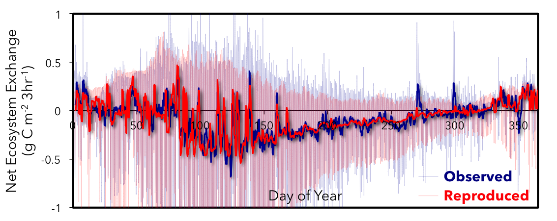
Figure 2. The observed net ecosystem exchange (NEE) (blue) and reproduced NEE (red) shown at the 3-hourly time step with daily moving window overlaid for a single year from the Tonzi Ranch AmeriFlux/FLUXNET site (Baldocchi and Ma, 2013)
Data Acquisition, Materials, and Methods
Global gridded model output data (GPP, Re, and NEE) for net ecosystem exchange (NEE) of CO2 fluxes between the land and atmosphere were downscaled to 3-hourly time steps from monthly resolution. Models were from MsTMIP, version 1, (Huntzinger et al., 2013) and included: 1) BIOME_BGC, 2) CLM, 3) CLM4VIC, 4) CLASS_CTEM, 5) DLEM, 6) GTEC, 7) ISAM, 8) LPJ, 9) ORCHIDEE, 10) SIB3, 11) SIBCASA, 12) TEM6, 13) TRIPLEX-GHG, 14) VEGAS, and 15) VISIT. Four ensemble products were also included: 1) un-weighted (naive) ensemble mean, 2) un-weighted (naive) ensemble standard deviation, 3) weighted (optimal) ensemble mean, and 4) weighted (optimal) ensemble standard deviation.
The four ensemble products were derived as described in Schwalm et al. (2015). The un-weighted (naive) ensemble outputs are the result of combining ensemble models to a single-integrated mean value where each model is weighted equally. The weighted (optimal) ensemble outputs are the result of combining ensemble models to a single-integrated mean value where each model's weight ("Reliability Factor”) was derived using reliability ensemble averaging (REA). The "Reliability Factors" are not included in standard MsTMIP global model outputs.
Downscaling
The general downscaling approach follows Olsen and Randerson (2004) with modifications. The logic takes the components of NEE, i.e., gross primary production (GPP) and ecosystem respiration (Re), and links them with incident shortwave solar radiation (I) and surface air temperature (Ta), respectively. I and Ta are provided at 6-hourly time steps from CRU-NCEP (Wei et al., 2014), which were interpolated to 3-hourly time steps following cosines of solar zenith angle for I and linear interpolation for Ta. Hence, GPP and Re are temporally downscaled to 3-hourly, and re-combined to form NEE at 3-hourly time steps.
The 6-hourly to 3-hourly solar zenith angle cosine interpolation follows this equation:
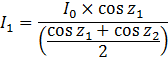
where z is solar zenith angle and / is in units of W m-2 . As an example, if the 0-6 hour /0 was 100 W m-2, and the 0-3 hour z1 was 0 (i.e., cos(z1) = 1) and the 3-6 hour z2 was 60 (i.e., cos(z2) = 0.5), then the 0-3 hour I1 would be 133.3 W m-2, and the 3-6 hour I2 would be 66.7 W m-2.
To scale GPP and Re to 3-hourly time steps, the steps used by Olsen and Randerson (2004) were followed with modifications starting first with the calculation of scale factors based on I and Ta:
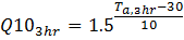
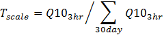

where Q10 is the temperature dependency of Re, and Ta is in degrees Celsius (converted from Kelvin, as provided by CRU-NCEP). Note that Olsen and Randerson (2004) originally used time integral periods of calendar months, but it was observed that this caused unrealistic distinct shifts between months. Instead, the integral period was modified to a 30-day moving window. For the first 15 days of January of the record and the last 15 days of December of the record, the last 15 days of December and the first 15 days of January were used, respectively, within the first (2004) and last (2010) years to complete the 30-day window.
The 3-hourly resolution scale factors are then multiplied by GPP and Re, respectively, for each 3-hourly time step each month:

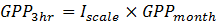
Remonth and GPPmonth were modified from Olsen and Randerson (2004) to be given at a 3-hourly time step, linearly interpolated to 3-hourly time steps based on the present, previous, and subsequent month, maintaining the original units (g C m-2 mo-1). Re3hr and GPP3hr are in units of g C m-2 3hr-1. This modification avoided using the same monthly value for the multiplier for all 3-hourly time steps per month as per Olsen and Randerson (2004), and instead provided a smooth transition from one month to the next. The result of this modification was to eliminate a “ramping” effect whereby values would, for example, increase steadily within a month, then suddenly shift to a new starting point at the beginning of the next month. Note that the original nomenclature of Olsen and Randerson (2004) used [(2 x NPPmonth ) - NEPmonth ] in place of Remonth, and in place of GPPmonth, where NPP is net primary production (GPP minus autotrophic respiration) and NEP is net ecosystem production (approximately equivalent to the inverse sign of NEE, with caveats (Hayes and Turner 2012)). The assumption here, therefore, is that GPP= 2 x NPP and Re = (2 x NPP) - NEP. The Re assumption misses CO2 emissions other than respiration, e.g., fire, which were corrected for at a later step.
The initial NEE calculation simply subtracts GPP from Re:
NEE3hr = Re3hr - GPP3hr
where NEE3hr is calculated in units of g C m-2 3hr-1. However, we applied an additional units conversion for the publicly available data to kg C km-2 s-1, as these units are more readily ingestible by atmospheric inversion models (Deng et al., 2014).
Because the downscaling approach uses Re as the primary CO2 efflux term, other ecosystem CO2 loss components, such as fire and other disturbances (Hayes and Turner, 2012),were excluded in the downscale. Hence, the sum of the downscaled 3-hourly NEE fluxes in a given month did not necessarily equal the original monthly NEE flux. So, a per-pixel correction was included whereby: I) the difference was calculate between the sum of the downscaled 3-hourly NEE in a given month and the original monthly NEE; II) that difference was divided by the total 3-hourly time steps in the month, and III) that difference was added to each 3-hourly NEE flux. In so doing, the sum of the downscaled 3-hourly NEE fluxes subsequently summed exactly to the original monthly NEE.
Temporally Downscaled Output Products -- Spatial Upscaling
All input data were at a spatial resolution of 0.5 degree x 0.5 degree (latitude/longitude), therefore, the 3-hourly NEE output have been provided in 0.5 degree x 0.5 degree. Two additional sets of spatially upscaled NEE output are also provided in 2.0 degree x 2.5 degree and 4.0 degree x 5.0 degree to facilitate ingestion by the atmospheric modeling community (e.g., forward modeling versus flux inversion). To generate the coarser resolution data: I) Each pixel value was multiplied by the land area of that pixel; II) the flux was summed from all pixels that represent one pixel in coarser resolution (e.g., 8 x 10 pixels from 0.5 degree x 0.5 degree comprise 1 pixel in 4.0 degree x 5.0 degree); III) calculated the total area covered by the pixels summed in step II; and, IV) the value in step II was divided by the value in step III. The regridding preserved the total sum flux of the finer grid cells as well as the total global flux. A file is provided containing the land area contained in each latitudinal band for each of the three resolutions. Note that the northern and southern most latitudinal bands for the 2.0 degree x 2.5 degree resolution are 1.0 degree x 2.5 degree, and for the 4.0 degree x 5.0 degree they are 2.0 degree x 5.0 degree. This inconsistency was created for facilitation into the atmospheric models.
Data Access
These data are available through the Oak Ridge National Laboratory (ORNL) Distributed Active Archive Center (DAAC).
CMS: Modeled Net Ecosystem Exchange at 3-hourly Time Steps, 2004-2010
Contact for Data Center Access Information:
- E-mail: uso@daac.ornl.gov
- Telephone: +1 (865) 241-3952
References
Baldocchi, D. and Ma, S. How will land use affect air temperature in the surface boundary layer? Lessons learned from a comparative study on the energy balance of an oak savanna and annual grassland in California, USA, Tellus B, 65, 2013.
Baldocchi, D., Falge, E., Gu, L. H., Olson, R. J., Hollinger, D., Running, S. W., Anthoni, P. M., Bernhofer, C., Davis, K., Evans, R., Fuentes, J., Goldstein, A., Katul, G., Law, B. E., Lee, X. H., Malhi, Y., Meyers, T., Munger, W., Oechel, W., U, K. T. P., Pilegaard, K., Schmid, H. P., Valentini, R., Verma, S., Vesala, T., Wilson, K., and Wofsy, S. C.: FLUXNET: A new tool to study the temporal and spatial variability of ecosystem-scale carbon dioxide, water vapor, and energy flux densities, Bulletin of the American Meteorological Society, 82, 2415-2434, 2001.
Deng, F., Jones, D., Henze, D., Bousserez, N., Bowman, K., Fisher, J., Nassar, R., O'Dell, C., Wunch, D., and Wennberg, P.: Inferring regional sources and sinks of atmospheric CO 2 from GOSAT XCO 2 data, Atmospheric Chemistry and Physics, 14, 3703-3727, 2014.
Hayes, D. and Turner, D. The need for “apples-to-apples” comparisons of carbon dioxide source and sink estimates, Eos, Transactions American Geophysical Union, 93, 404-405, 2012.
Huntzinger, D., Schwalm, C., Michalak, A., Schaefer, K., King, A., Wei, Y., Jacobson, A., Liu, S., Cook, R., Post, W., Berthier, G., Hayes, D., Huang, M., Ito, A., Lei, H., Lu, C., Mao, J., Peng, C., Peng, S., Poulter, B., Riccuito, D., Shi, X., Tian, H., Wang, W., Zeng, N., Zhao, F., and Zhu, Q.: The North American Carbon Program Multi-scale synthesis and Terrestrial Model Intercomparison Project-Part 1: Overview and experimental design, Geoscientific Model Development, 6, 2121-2133, 2013.
Olsen, S. C. and Randerson, J. T. Differences between surface and column atmospheric CO2 and implications for carbon cycle research, Journal of Geophysical Research: Atmospheres (1984–2012), 109, 2004.
Schwalm, C. R., D. N. Huntzinger, J. B. Fisher, A. M. Michalak, K. Bowman, P. Ciais, R. Cook, B. El-Masri, D. Hayes, M. Huang, A. Ito, A. Jain, A. W. King, H. Lei, J. Liu, C. Lu, J. Mao, S. Peng, B. Poulter, D. Ricciuto, K. Schaefer, X. Shi, B. Tao, H. Tian, W. Wang, Y. Wei, J. Yang, and N. Zeng (2015), Toward “optimal” integration of terrestrial biosphere models. Geophys. Res. Lett., 42, 4418–4428. doi: 10.1002/2015GL064002.
Wei, Y., Liu, S., Huntzinger, D., Michalak, A., Viovy, N., Post, W., Schwalm, C., Schaefer, K., Jacobson, A., and Lu, C. The North American Carbon Program Multi-scale Synthesis and Terrestrial Model Intercomparison Project–Part 2: Environmental driver data, Geoscientific Model Development, 7, 2875-2893, 2014.