ABoVE: Surface Water Extent, Boreal and Tundra Regions, North America, 1991-2011

This data set provides the location and extent of surface water (open water not including vegetated wetlands) for the entire Boreal and Tundra regions of North America for three epochs, centered on 1991, 2001, and 2011. Each of the products were generated with at least three years of ice-free Landsat imagery. The data are at 30-m resolution and were derived from time series of Landsat 4 and 5 Thematic Mapper (TM) data and Landsat 7 Enhanced Thematic Mapper (ETM+) covering all of Alaska and all provinces of Canada. The overall goal was to generate a map of the nominal extent of water for a given epoch, where nominal is neither the maximum nor the minimum but rather a representative extent for that time period.

To aid the use of the product a quality assurance (QA) layer was generated for each data file (map). These data provide additional information regarding the source of values in the water extent maps and the confidence in the extent value determined by the number of water image observations in the probability of water.

There are 78 data files in GeoTIFF (.tif) format with this data set. This includes 39 surface water body data files and 39 QA files, one for each of the data files.

 

Project: ABoVE

This data set provides the location and extent of surface water (open water not including vegetated wetlands) for the entire Boreal and Tundra regions of North America for three epochs, centered on 1991, 2001, and 2011. Each of the products were generated with at least three years of ice-free Landsat imagery. The data are at 30-m resolution and were derived from time series of Landsat 4 and 5 Thematic Mapper (TM) data and Landsat 7 Enhanced Thematic Mapper (ETM+) covering all of Alaska and all provinces of Canada. The overall goal was to generate a map of the nominal extent of water for a given epoch, where nominal is neither the maximum nor the minimum but rather a representative extent for that time period.

To aid the use of the product a quality assurance (QA) layer was generated for each data file (map). These data provide additional information regarding the source of values in the water extent maps and the confidence in the extent value determined by the number of water image observations in the probability of water.

The three epochs are centered and the temporal range of the data set for each epoch is as follows:

1991: 1990-01-01 to 1992-12-31; 2001: 2000-01-01 to 2002-12-31; 2011: 2010-01-01 to 2012-12-31

Note: This data set will be expanded for south and east of the Hudson Bay in the future.

The Arctic-Boreal Vulnerability Experiment (ABoVE) is a NASA Terrestrial Ecology Program field campaign taking place in Alaska and western Canada between 2016 and 2021. Climate change in the Arctic and Boreal region is unfolding faster than anywhere else on Earth, resulting in reduced Arctic sea ice, thawing of permafrost soils, decomposition of long-frozen organic matter, widespread changes to lakes, rivers, coastlines, and alterations of ecosystem structure and function. ABoVE seeks a better understanding of the vulnerability and resilience of ecosystems and society to this changing environment.

Related Publication:

Carroll, M., Wooten, M., DiMiceli, C., Sohlberg, R. and Kelly, M., 2016. Quantifying surface water dynamics at 30 meter spatial resolution in the North American high northern latitudes 1991–2011. Remote Sensing, 8(8), p.622. https://doi.org/10.3390/rs8080622

Spatial Coverage: 

Boreal and Tundra regions of North America -- covering all of Alaska and all provinces of Canada

ABoVE Site Designation:

Domain: Core and extended ABoVE regions

State/territory: All provinces of Canada and the State of Alaska

Grid cells: Ah00v00, Ah00v01, Ah01v00, Ah01v01, Ah01v02, Ah02v00, Ah02v01, Ah02v02, Ah02v03, Ah03v00, Ah03v01, Ah03v02, and Ah03v03

Spatial Resolution: 30 meter

Temporal Coverage: Decadal time steps (1991, 2001, and 2011 epochs)

Temporal Resolution: Annual -- representative extent for the epoch

Study Area: (all latitudes and longitudes given in decimal degrees)

Site (Region)	Westernmost Longitude	Easternmost Longitude	Northernmost Latitude	Southernmost Latitude
ABoVE study regions, including Canada and Alaska	-177.474	-53.9489	82.37278	41.71167

 

Data File Information

There are 78 data files in GeoTIFF (.tif) format with this data set. Since the data are in GeoTIFF format intended for display as maps, they may also be referred to as maps. This includes 39 files of surface water data and 39 “QA” files, one for each of the surface water files. The QA files provide additional information regarding the source of values in the data files or the confidence in the water value determined by the number of water observations in the probability of water. The overall goal was to generate a map of the nominal extent of water for a given epoch, where nominal is neither the maximum nor the minimum but rather a representative extent for that time period.

The files are named by year and grid tiles generated for this study (Figure 2) based on the Canada Albers Equal Area projection with equal sized “tiles” modeled after the MODIS labeling convention with horizontal and vertical offsets, thus there are two files per area and per year (non-QA and QA files). This grid is in coordination with the ABoVE project study areas. The study area covered 13 grid cells.

 

 

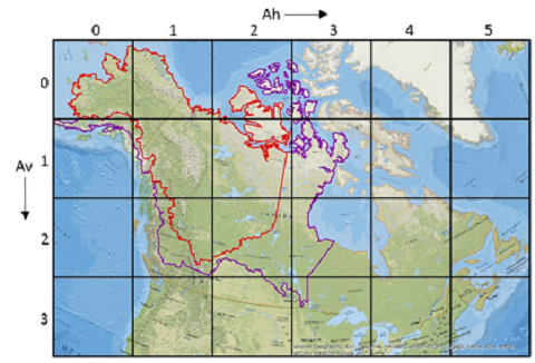
Figure 2. Proposed ABoVE reference grid for use with large area products. Based conceptually on the MODIS tiling scheme but utilizing Canada Albers Equal Area projection (Carroll et al., 2016).

 

Example file names:

ABoVE_Water_h00v00_1991.tif  and ABoVE_Water_h00v00_1991_QA.tif (h00v00 refers to the top left corner grid cell in Figure 2)

ABoVE_Water_h02v00_2001.tif and ABoVE_Water_h02v00_2001_QA.tif (h02v00 refers to the first row of cells, third cell from the left in Figure 2)

 

GeoTIFF Spatial Data Properties, all files

Spatial Representation Type: Raster

Data Type: byte

Number of Bands:1

Number Columns: 3600

Column Resolution: 30 meter

Number Rows: 3600

Row Resolution: 30 meter

Fill value: -3.4E+38

DATUM: North American Datum 1983

Grid cell extents in the projected coordinate system and in decimal degrees:

Grid cells	Min_x	Min_y	Max_x	Max_y	Decimal degrees-West	Decimal degrees-East	Decimal degrees-North	Decimal degrees-South
h00v00	-3400020	3560000	-2320020	4640000	-177.474	-148.288	69.27111	56.08472
h00v01	-3400020	2480000	-2320020	3560000	-160.864	-135.932	63.44056	49.86417
h01v00	-2320020	3560000	-1240020	4640000	-167.83	-128.593	77.25417	63.44056
h01v01	-2320020	2480000	-1240020	3560000	-148.288	-119.288	69.1525	56
h01v02	-2320020	1400000	-1240020	2480000	-135.932	-114	60.38972	47.67778
h02v00	-1240020	3560000	-160020	4640000	-147.915	-100.559	82.37278	69.1525
h02v01	-1240020	2480000	-160020	3560000	-128.593	-99.1186	71.88111	60.38972
h02v02	-1240020	1400000	-160020	2480000	-119.288	-98.3728	62.27111	51.22028
h02v03	-1240020	320000	-160020	1400000	-114	-97.9319	52.69472	41.71167
h03v00	-160020	3560000	919980	4640000	-104.407	-53.9489	82.37278	70.35583
h03v01	-160020	2480000	919980	3560000	-100.559	-70.9658	71.88111	61.23722
h03v02	-160020	1400000	919980	2480000	-99.1186	-78.4067	62.27111	51.89806
h03v03	-160020	320000	919980	1400000	-98.3728	-82.4914	52.69472	42.25417

 

Cell value attributes for map files:

0 - Land

1 - Water

2 - Probable water in Alaska 1991 tiles

255 - No data or outside ABoVE study domain, fill applied

 

Cell value attributes for QA files:

0 - Land

1 - High Confidence Water (probability >= 50% and n >5)

2 - Lower Confidence Water (probability >= 50% and 2<n<5)

3 - Ocean mask applied

4 - Fill based on 2001 and 2011

255 - No data or outside ABoVE study domain, fill applied

 

 

The Arctic and Boreal Vulnerability Experiment (ABoVE) will conduct multi-disciplinary studies to explore and quantify the linkages between all of the individual components of the ecosystem. One common thread identified in the final report for the scoping study for ABoVE was the need for maps of the location, extent and dynamics of surface water to connect the different disciplines. These maps will allow consistent evaluation of the extent of surface water through time in ways that were not previously possible (Carroll et al., 2016).

In addition to the QA data products provided with this data set as described in Section 5, several comparisons with existing land cover classification products were undertaken.

The ABoVE Water Map (AWM) data products were compared to the data in two global maps that include water as a class and are generated from Landsat data at 30-m spatial resolution, namely Globe Land 30 (GL30) (Zheng 2014) and the GLCF Inland Surface Water (GIW) (Feng et al. 2015). These maps were generated with Landsat data primarily from the Geocover or Global Land Survey (GLS) data collections and were essentially calculated with a single Landsat observation representing a single point in time, ~2001 for GIW and ~2010 for GL30. A per pixel analysis was performed with the AWM data to the water class from the GL30 land cover map and the GIW map. The GL30 and GIW products were mosaicked into the ABoVE projection and tile grid to facilitate comparison (Carroll et al., 2016).

The results for the comparison of data in the AWM products to GL30 and the AWM to GIW indicated large differences between the products and that this difference varies from tile to tile. Overall the majority of the differences come in the extent of water bodies where the GL30 over-estimates the size of the water bodies because it only uses a single input observation. This effect is pronounced on rivers where normal fluvial processes cause the river channel to meander. There are specific instances where entire water bodies are present in the AWM and not in GL30 and vice versa but these are limited in number (Carroll et al., 2016).

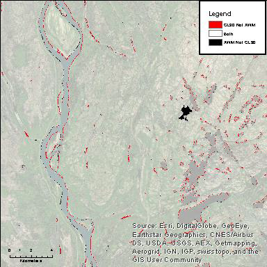
Figure 3. Image from central Canada shows differences between AWM and GL30 water coverage. Red shows areas where GL30 shows water and AWM does not, while black shows areas where AWM shows water and GL30 does not. Note this primarily occurs on the margins of water bodies but some instances of complete water bodies do occur, i.e. the large lake in the center of the image (Carroll et al., 2016).

Method verification with 1.84-m WorldView 2 data shows 95% accuracy in water bodies that are shown in the AWM and a 36% omission rate, primarily among lakes smaller than 1 Landsat pixel. The AWM shows 25% more water bodies than the Global Land Cover 30 (30 m Landsat based land cover product) from the same time period.

There are still some burn scars that trigger false positive water detection in all products but this effect is minimized in the AWM. Currently these issues are being addressed and may be improved in a future release of AWM (Carroll et al., 2016).

Site description

The continental surface of the Arctic and Boreal regions of the world is critical to understanding components of the ecosystem as well as the Arctic system as a whole. These landscapes are dominated by a heterogeneous land surface dotted with lakes, ponds and wetlands (Carroll et al., 2011; Downing et al., 2006; Smith et al., 2005). The primary region of study for this project is the ABoVE study region shown in Figure 4 but data cover all of Alaska and Canada.

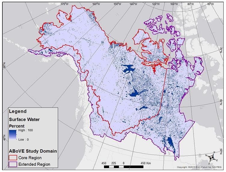
Figure 4.  ABoVE study area in northern North America overlain with a subset of the Global 250m Water Map (Carroll et al., 2016).

Methods

Landsat Data

This data set provides the location and extent of surface water (open water not including vegetated wetlands) for the entire Boreal and Tundra regions of North America for three epochs (1991, 2001, and 2011) in GeoTIFF format for display as maps. The data are at 30-m resolution and were derived from a time series of Landsat 4 and 5 Thematic Mapper (TM) data and Landsat 7 Enhanced Thematic Mapper (ETM+). The data were acquired from the US Geological Survey Eros Data Center through the ESPA ordering interface (https://espa.cr.usgs.gov/).

The data from 2000 to present for Landsat 5 and 7 are of good quality and relatively high repeat coverage with a minimum of 30 individual dates per scene for most scenes. The data for the 1990-1992 epoch are primarily from Landsat 5, supplemented with Landsat 4 in Alaska where data density is thinner. Data acquisition strategies in the early 1990’s resulted in a limited archive of data over Alaska at this time (Goward et al. 2006). 

All Landsat scenes were acquired and processed regardless of cloud coverage. This decision was based on experience with MODIS data where even a scene that is 80% - 90% cloudy can have clear observations of certain areas. Using all of the available observations can increase the total density of the observations in any given area to get a consensus result. This method is enhanced in the Arctic due to the high degree of overlap between adjacent Landsat path/rows. By processing all of the available overlapping scenes it becomes possible to increase the total number of observations, which minimized the impacts of clouds and weather related phenomena such as drought and flood (Carroll et al., 2016).

Classification per scene

All Landsat scenes were processed through a decision tree image classification scheme to generate an output with six classes: Water, Vegetated Land, Bare Ground, Snow/Ice, Cloud, Cloud Shadow. Quality assurance flags in the surface reflectance files provide an indication of cloudy and cloud shadow pixels and were used in the classification process. This process was modeled after the approach taken to generate the Global 250m Water Map with Moderate Resolution Imaging Spectro-radiometer (MODIS) data (Carroll et al., 2009) and a host of other land cover mapping efforts. The algorithm was designed to be conservative in the labeling of water in order to minimize the errors of commission (i.e. labeling land as water). The overall goal was to generate a map of the nominal extent of water for a given epoch, where nominal is neither the maximum nor the minimum but rather a representative extent for that time period (Carroll et al., 2016).

Sum of observations per scene (path/row)

The classification results have six classes, as described above. Thematic layers were extracted (i.e. one of the classes, water or land for example) and summary results were created for a particular path/row using all of the available dates within an epoch. The result was a value from 0 to “n” where “n” is the total number of dates that were available for that path/row for that particular theme. This process was repeated for each theme as necessary to produce the desired result.

In order to generate a unified product for the entire study region, the individual path/row results needed to be combined into a common projection and grid. In coordination with the ABoVE project office and other pre-ABoVE projects, it was decided to generate a grid based on the Canada Albers Equal Area projection with equal sized “tiles” modeled after the MODIS labeling convention with horizontal and vertical offsets (Figure 2). To take advantage of the significant overlap between path/rows it was necessary to mosaic with intermediate steps to map the individual scenes into a series of tiles with non-overlapping scenes and then sum the resulting tiles. In this way all information was retained from all Landsat observations which maximized the chance for clear observations and raises confidence level in the final product (Carroll et al., 2016).

Generation of final maps (data available in GeoTIFF format for display as maps)

The thematic data layers in large area tiles represent sum of water, sum of land, etc. The desired final map is a binary representation of “water” and “not water”. The thematic layers were used to generate a probability of water as:

Pw=(W/(W+L))

where Pw is probability of water; W is sum of water observations; and L is sum of land observations. The final map was generated by labeling anything with 50% or greater probability of water as water and labeling anything else as land or no data. Anything else is labeled as land or no data.

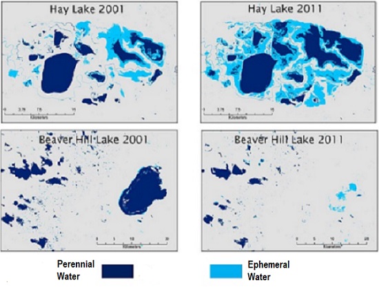
Figure 5.  AWM for 2001 and 2011 for Hay Lake and Beaver Hill Lake in Canada. Hay Lake has clearly expanded over this time frame while Beaver Hill Lake has diminished (Carroll et al., 2016).

Generation of QA data

To aid the use of the product a quality assurance (QA) layer was generated for each data file (map). These data provide additional information regarding the source of values in the water extent maps or the confidence in the water value determined by the number of water observations in the probability of water.

Ocean mask

An ocean mask was created by combining the data in the MODIS Collection 6 water map (Carroll et al. 2009) and a consensus coastline generated by combining the data in the three ABoVE water maps (1991, 2001, and 2011). The goal was to create a mask to fill in the permanent ocean waters where the map would otherwise have been intermittent due to unavailable Landsat scenes, moving sea ice, or other so that the final map was more aesthetically pleasing. Below are the general steps used to make the mask:

• All three years of data in the ABoVE Water Maps (AWM) were mapped to single output allowing maximum extent of coastline
• MODIS water map data were converted to ABoVE tile map outputs
• Ocean class was identified from MODIS water map data
• Areas were selected from AWM data that intersected MODIS water map oceans
• The land in the AWM data was buffered by 10 Landsat pixels (300-m) to allow for shifting coastlines (Carroll et al., 2016)

The resulting data were applied to each of the ABoVE water maps to yield a more aesthetic result. The areas that have been mapped with the ocean mask are indicated in the QA layer so a user can understand how and where that was applied. The coastlines within 300 m of the consensus coastline were buffered and not masked to allow the user to see differences in the coastline through time (Carroll et al., 2016).

Terrain shadow mask

Terrain shadow was found to be the primary source of false identification of water in the final water maps. A mask was generated using the Digital Elevation Model (DEM) from the Global Land Survey project where slope was greater than or equal to five degrees and the elevation was over 450 m. The elevation threshold was used to minimize the impact of the slope threshold on rivers in lowlands. This mask was applied to all tiles to address the problem of terrain shadows and follows previous work addressing similar problems of terrain shadow being confused with water (Klein et al. 2015).

Alaska 1991 epoch

In most areas there were at least twenty observations for any given pixel. However for Alaska in the 1991 epoch there are fewer than seven observations for most of the state, and in some cases there were only one or two observations. This is caused by the lack of a receiving station that could collect the data at the time of overpass and is well documented (Goward et al. 2006). The map that was generated for the 1991 epoch for Alaska is significantly impacted by the lack of input data. Consequently, a procedure was developed to fill in the holes in order to make a complete map for this epoch:

• A mask was generated of location of water in both 2001 epoch and 2011 epoch.
• Any water observation from 1991 was selected that was under the mask disregarding probability of water and minimum number of water observations rules.
• In the water mask, the new values were set as water, and QA was set to “2”  to indicate that the values are low confidence and should be used with significant caution.
• Where 2001 and 2011 still show water and there are no observations from 1991, the water map value was set to “2” to indicate probable water and the QA code was set to “4” to indicate “fill based on 2001 and 2011”.

This procedure improved the appearance of the map but the quality of the data is still significantly lower than it is for other epochs and elsewhere in the 1991 epoch. The affected tiles are h00v00, h00v01, and h01v00 with the most affected areas located in the far west and south west in Alaska. Under no circumstances should the water map with QA value “4” be used to indicate change; these values are included simply for aesthetic purposes. Water values with a QA value of “2” should be used with caution when performing change analysis and should be indicated in the results as “possible” change (Carroll et al., 2016).

 

Carroll, M.L., Townshend, J.R., DiMiceli, C.M., Noojipady, P., and Sohlberg, R.A. (2009). A new global raster water mask at 250 m resolution. International Journal of Digital Earth, 2, 291-308

Carroll, M.L., Townshend, J.R.G., DiMiceli, C.M., Loboda, T., and Sohlberg, R.A. (2011). Shrinking lakes of the Arctic: Spatial relationships and trajectory of change. Geophysical Research Letters, 38.

Carroll, M., Wooten, M., DiMiceli, C., Sohlberg, R. and Kelly, M., 2016. Quantifying surface water dynamics at 30 meter spatial resolution in the North American high northern latitudes 1991–2011. Remote Sensing, 8(8), p.622. https://doi.org/10.3390/rs8080622

Downing, J.A., Prairie, Y.T., Cole, J.J., Duarte, C.M., Tranvik, L.J., Striegl, R.G., McDowell, W.H., Kortelainen, P., Caraco, N.F., Melack, J.M., and Middelburg, J.J. (2006). The global abundance and size distribution of lakes, ponds, and impoundments. Limnology and Oceanography, 51, 2388-2397.

Feng, M., Sexton, J.O., Channan, S., and Townshend, J.R. (2015). A global, high-resolution (30-m) inland water body dataset for 2000: first results of a topographic–spectral classification algorithm. International Journal of Digital Earth, 1-21.

Goward, S., Arvidson, T., Williams, D., Faundeen, J., Irons, J., and Franks, S. (2006). Historical Record of Landsat Global Coverage. Photogrammetric Engineering & Remote Sensing, 72, 1155-1169.

Klein, I., Dietz, A., Gessner, U., Dech, S., and Kuenzer, C. (2015). Results of the Global WaterPack: a novel product to assess inland water body dynamics on a daily basis. Remote Sensing Letters, 6, 78-87.

Smith, L.C., Sheng, Y., MacDonald, G.M., and Hinzman, L.D. (2005). Disappearing Arctic lakes. Science, 308, 1429.

Zheng, X. (2014). GlobeLand 30. In N.G.C.o. China (Ed.). Beijing, China.