A USER'S GUIDE TO THE VEMAP PHASE I DATABASE

November 1996 (revised December 1998)

Nan Rosenbloom
Timothy G.F. Kittel

To accompany CDROM and World Wide Web versions of:

THE VEMAP PHASE I DATABASE:

AN INTEGRATED INPUT DATASET FOR ECOSYSTEM AND VEGETATION MODELING
FOR THE CONTERMINOUS UNITED STATES

T.G.F. Kittel, N.A. Rosenbloom, T.H. Painter, D.S. Schimel, H.H. Fisher,
A. Grimsdell, VEMAP Participants, C. Daly, and E.R. Hunt, Jr.

Ecosystem Dynamics and the Atmosphere Section
Climate and Global Dynamics Division
National Center for Atmospheric Research

and

Climate System Modeling Program
University Corporation for Atmospheric Research

Data Citation:

This data set should be cited as follows:

Kittel, T. G. F., N. A. Rosenbloom, T. H. Painter, D. S. Schimel, H. H. Fisher, A. Grimsdell, VEMAP Participants, C. Daly, and E. R. Hunt, Jr. 2002. VEMAP Phase I Database, revised. Available online [http://daac.ornl.gov/] from the ORNL Distribued Active Archive Center, Oak Ridge National Laboratory, Oak Ridge, Tennessee, U.S.A.

List of Tables and Figures

Table 1 Datasets available on the VEMAP CDROM, Web site, and FTP site
Table 2 VEMAP grid corners defining the minimum bounding rectangle
Table 3 Format of data records in site files
Table 4a Number of Background cells (excluding wetlands)
Table 4b Number of Background cells (including wetlands)
Table 5 Geographic variables
Table 6 Climate variables
Table 7 Soil variables
Table 8 Vegetation variable name code and description
Table 9 VEMAP vegetation types
Table 10 Availability of climate variables for each climate scenario
Table A3.1 Aggregation of Küchler vegetation types to VEMAP vegetation types
Table A3.2 Küchler Vegetation Type Names and Identifying Codes
Figure 1 Layout of the VEMAP gridded array
Figure 2 Schematic illustration of relationships among radiation variables in the climate dataset

1 INTRODUCTION
- 1.1 VEMAP and the VEMAP Database
- 1.2 Citations and User Access Acknowledgments
2 DATA FILE ACCESS
3 THE VEMAP GRID
4 FILE STRUCTURE
5 SCALING FACTORS, BACKGROUND VALUES, AND LANDCOVER MASK
6 ROAD MAP TO FILE AND VARIABLE DESCRIPTIONS
7 GEOREFERENCING VARIABLES AND CELL AREAS
8 DAILY, MONTHLY, AND ANNUAL CLIMATE DATASETS
9 SOILS
10 VEGETATION
11 CLIMATE CHANGE SCENARIOS
12 SITE FILES
- 12.1 Site File Content and Structure
- 12.2 Site File Naming Protocol
13 ACKNOWLEDGMENTS
14 CONTACTS
15 REFERENCES
A1 APPENDIX 1: CDROM AND FTP SITE DIRECTORY STRUCTURE
A2 APPENDIX 2: DETERMINATION OF ABSOLUTE SOIL AREA FOR EACH CELL
- A2.1 Absolute Area for Soil Modes and Components
- A2.2 Application to Model Outputs
A3 APPENDIX 3: AGGREGATION OF KÜCHLER VEGETATION CODES TO VEMAP VEGETATION TYPES
A4 APPENDIX 4: STATE IDENTIFICATION NUMBERS

1 INTRODUCTION

1.1 VEMAP and the VEMAP Database

The Vegetation/Ecosystem Modeling and Analysis Project (VEMAP) is an ongoing multi-institutional, international effort addressing the response of biogeography and biogeochemistry to environmental variability in climate and other drivers in both space and time domains. The objectives of VEMAP are the intercomparison of biogeochemistry models and vegetation-type distribution models (biogeography models) and determination of their sensitivity to changing climate, elevated atmospheric carbon dioxide concentrations, and other sources of altered forcing. The VEMAP exercise allows us to identify important commonalties and differences among model controls and responses. Where the models differ, the comparison highlights areas of uncertainty or error and identifies problems for future research. Inter-model differences also help to quantify the uncertainty in modeled responses to changing climate and other drivers.

The completed Phase I of the project was structured as a sensitivity analysis, with factorial combinations of climate (current and projected under doubled CO₂), atmospheric CO₂, and mapped and model-generated vegetation distributions. The highly structured nature of the intercomparison allowed rigorous analysis of results, while constraining the range of questions explored. Maps of climate, climate change scenarios, soil properties, and potential natural vegetation were prepared as common boundary conditions and driving variables for the models (Kittel et al. 1995). As a consequence, differences in model results arose only from differences among model algorithms and their implementation rather than from differences in inputs. Results from VEMAP I are reported in VEMAP Members (1995) and selected files are available through UCAR's anonymous FTP server (see Section 2.3). Abstracts describing the six modeling groups participating in VEMAP Phase I can be found under the subdirectory /docs.

The VEMAP input database for the Phase I model intercomparison is documented in this Technical Note. It includes compiled and model-generated datasets of long-term mean climate, soils, vegetation, and climate change scenarios for the conterminous United States. The data are on a 0.5deg. latitude/longitude grid. There are both daily and monthly representations of the mean climate. The climate data and climate change scenarios are presented in both gridded and time-sequential format. We developed the time-sequential, "site" file format to facilitate extractions of information for individual grid cells (Sections 4.3 and 12).

1.2 Citations and User Access Acknowledgments

The citations for the VEMAP database are:

Kittel, T.G.F., N.A. Rosenbloom, T.H. Painter, D.S. Schimel, H.H. Fisher, A. Grimsdell, VEMAP Participants[1], C. Daly, and E.R. Hunt, Jr. (1998) The VEMAP Phase I Database: An Integrated Input Dataset for Ecosystem and Vegetation Modeling for the Conterminous United States. Available online at [http://www.daac.ornl. gov/] from the ORNL Distribued Active Archive Center, Oak Ridge National Lab oratory, Oak Ridge, Tennessee, U.S.A.

Development of the VEMAP database was supported by NASA Mission to Planet Earth, Electric Power Research Institute (EPRI), USDA Forest Service Southern Region Global Change Research Program, and NSF-ATM Climate Dynamics Program through the University Corporation for Atmospheric Research's Climate System Modeling Program.

2 DATA FILE ACCESS

The VEMAP database is available on CDROM, through the Internet on the DAAC Web site, or via anonymous FTP from the DAAC anonymous FTP server.

2.1 CDROM

The VEMAP database CDROM contains the complete set of input files used for the VEMAP model intercomparison. We present the monthly data files in both gridded format (SVF) and time-sequential columnar format (site files), and the daily variables in binary format. Table 1 contains a list of the files available on the CDROM and Appendix A1 provides an overview of the CDROM directory structure. A README file resides under each subdirectory describing the files within that directory. We have included example postscript images under the subdirectory /images.

Table 1. Datasets available on the VEMAP CDROM, Web site (www), and FTP site.

Category
File Structure
File Format
Access
Georeferencing
Gridded data
SVF*
CDROM, www, FTP
Monthly Climate
Gridded data
SVF
CDROM, www, FTP
Daily Climate
Sequential data
IEEE Binary
CDROM, www, FTP
Soil
Gridded data
SVF
CDROM, www, FTP
Vegetation
Gridded data
SVF
CDROM, www, FTP
Climate Scenarios
Gridded data
SVF
CDROM, www, FTP
Site
Sequential data
ASCII Columnar
CDROM, www, FTP
Bulk Transfer
Multiple files
UNIX Tarfiles
www, FTP
Phase I Model Results
Gridded data
SVF
www, FTP

*SVF = ASCII gridded "Single Variable Format" (see Section 4.1)

2.2 DAAC World Wide Web Site

The VEMAP files are accessible from the Internet. Using an Internet browser (e.g., Mosiac, Netscape, etc.), enter the URL:

http://daac.ornl.gov/

Note for Macintosh Users: If you are using an early version of Netscape on a Macintosh, you may have difficulty downloading files. In this case, it is advisable to obtain the VEMAP files via anonymous FTP from daac.ornl.gov/vemap-1 (see Section 2.3).

The VEMAP home page contains a short description of the VEMAP project and a directory to additional pages. To gain access to the VEMAP dataset from the VEMAP home page, click on "Access to the VEMAP Dataset" under the heading, "The VEMAP Dataset". A listing of available data files by dataset category is given in Table 1.

2.3 DAAC Anonymous FTP Server - daac.ornl.gov

To gain access to the VEMAP files via anonymous FTP from the DAAC FTP site, type:

> ftp daac.ornl.gov

Name: anonymous

Password: <your_login>

ftp> cd /vemap-1

ftp> cd <subdirectory>

ftp> get <filename>

Available datasets are listed in Table 1 and the FTP directory structure is presented in Appendix 1.

2.4 GNU Compressed UNIX Tarfiles (Web Site and FTP Site Only)

2.4.1 Description of GNU Compressed Tarfiles

We have archived multiple files into compressed UNIX tarfiles for more efficient data transfer. For example, all 12 gridded monthly maximum temperature files are stored in TX_MON.tar.gz (a .gz file suffix indicates that the tarfile has been compressed using the GNU software utility gzip, see below).

Tarfiles can be found on the FTP site under the subdirectory /tarFiles. To use these files, first FTP the desired tarfile to your home machine (remember to set the transfer mode to binary before FTP'ing the tarfiles). Then, decompress the .gz file and extract the archived files using the GNU gzip and tar commands appropriate to your machine. For example, on a UNIX system, type:

> gunzip <filename.gz>

> tar xvf <filename>

This process will create a complete set of files in your current local directory. The tarfiles frequently contain a considerable number of files and require sufficient space in your current directory. For a complete listing of the space required for the contents of each tarfile, download the file:

vemap-1/data/tarFiles/README.tarFiles

from daac.ornl.gov

Characteristic decompressed and/or extracted individual file sizes are:

Daily binary: ~4700 kBytes/file

Gridded SVF: ~33 kBytes/file

Columnar Site: ~370 kBytes/file

2.4.2 How to Obtain Free GNU Software

The gzip utility is provided by the Free Software Foundation GNU project. It is available for multiple system platforms, and may be freely downloaded from the Internet. The Macintosh gzip version is available at:

http://persephone.cps.unizar.es/general/gente/spd/gzip/gzip.html

UNIX and MS-DOS versions, along with other GNU software, can be found at:

ftp://prep.ai.mit.edu/pub/gnu/

2.4.3 Hints for Using gzip on Selected Systems

UNIX: To compress files, use the command gzip; gunzip will decompress a .gz file. The command man gzip will provide more information on how to use gzip.

MS-DOS: To compress files, use the command gzip; gzip -d will decompress a .gz file. The command gzip -h will provide more information on how to use gzip.

Macintosh: The Macintosh web site provides full instructions on how to use MacGzip.

3 THE VEMAP GRID

The grid used for the VEMAP coverage is a 0.5deg. latitude x 0.5deg. longitude grid covering the conterminous U.S. Grid edges are aligned with 1.0deg. and 0.5deg. latitude-longitude lines; grid centers are located at 0.25deg. and 0.75deg. latitude-longitude intersections. Latitude and longitude for each cell are included in the VEMAP dataset (Section 7.3).

The grid's minimum bounding rectangle (MBR) is defined by grid domain corners given in Table 2. The full 0.5deg. VEMAP grid contains 5520 cells, with 115 columns and 48 rows.

Table 2. VEMAP grid corners defining the minimum bounding rectangle (MBR).

Grid Position
Longitude*
Latitude
Lower Left Corner
-124.5deg.
25.0deg.
Upper Right Corner
-67.0deg.
49.0deg.

*Negative longitudes are degrees West.

4 FILE STRUCTURE

We use three file formats throughout the VEMAP dataset:

(1) ASCII SVF format for gridded monthly current climate, climate change scenarios, soils, vegetation, and georeferencing files.

(2) Binary time-sequential format for daily climate data. Each record contains the "characteristic year" of daily data for a grid cell (Section 8.3). Records are indexed by grid cell.

(3) ASCII column format for sequential monthly climate data and climate change scenarios. Each line presents 12 monthly values for a single grid cell. Records are indexed by grid cell (site files, Section 12).

4.1 SVF File Format

All gridded VEMAP data files are in an ASCII format based on, but not identical to, the SVF format specified by the GENAMAP Geographic Information System (GIS). Typical SVF files have 2 header lines followed by a 6-digit integer array. In contrast, VEMAP files have 5 header lines.

The first 2 lines are a VEMAP data access policy statement, followed by a blank line. These first 3 lines must be removed in order to convert the file to standard SVF format.

The 4th header line is a title line identifying the gridded variable and its units. For continuous data (i.e., non-categorical datasets), we also include the scale factor used to convert values to stored integers (Section 5.1). Division by this factor will restore the original value. Version number and revision date are also in the title line.

The 5th header line gives the gridded array's column and row indices (as four 6-digit integers): 1, 115 and 1, 48.

The header lines are followed by the gridded VEMAP integer array, which is dimensioned 115 columns x 48 rows (Section 3). The 6-digit integers in the VEMAP array include at least one blank space so that values in the file are space delimited. The array starts in the northwest corner of the grid, with the column index running west to east and row index running north to south (Fig. 1).

Figure 1. Layout of the VEMAP gridded array, with grid cell ID numbers.

Column

1

-to-

115

Row 1
1
2
3
4

...

115

116
117
118
119

...

230

231
...

-to-
.

.

.

48

...

5520

The full grid contains 5520 grid cells, 3261 of which are within the boundaries of the conterminous U.S. and predominantly covered by land (see Section 5.2). Background cells (ocean and inland water cells) are assigned the value of -9999.

4.2 Binary File Format

All daily variables are stored in IEEE binary format. We have provided a FORTRAN program to read the binary files:

/programs/biread.f

Each binary file contains 365 days of data for the 3261 grid cells with landcover in the U.S. Background grid cells are not included.

The files begin with two header lines containing information about the data. The first lists the variable name, units, scaling factor, and version number. The second describes the content of each data record with the following string:

gridpt|lon|lat|day (1->365)

The two header lines are followed by 3261 data records. Each record includes the grid point identifying number (ID), longitude, latitude, and a year's worth of scaled daily values. Only one year of data is given per grid cell, representing a "characteristic" year (see Section 8.3). Grid cell ID numbers begin at the top left corner of the grid and proceed left to right, top to bottom (Fig. 1).

Daily files on the NCAR FTP site or the WWW are available in GNU compressed format (Section 2.4) to speed FTP transmission.

4.3 ASCII Column Format for Site Files

Site files contain the monthly climate data and scenarios in column format, with each record containing 12 monthly values for a single variable. This time-sequential format was developed to facilitate data extraction for individual grid cells. Site files contain 8 header lines, beginning with a 2 line VEMAP data policy statement, followed by a blank line. The 4th header line is a title line identifying the gridded variable and its units. For continuous data (i.e., non-categorical datasets), we also include the scale factor used to convert values to stored integers (see Section 5.1). Division by this factor will restore the original value. Version number and revision date are also in the title line. The next 4 lines provide column headings for the data records.

In addition to the 12 monthly data values, each record contains auxiliary geographic information for each cell: grid cell ID, latitude, longitude, elevation, VEMAP vegetation type (Section 10 and Table 9), Küchler vegetation type (Appendix Table A3.2), and state identification number. The format of each data record is given in Table 3. VEMAP vegetation types listed in the site files are from version 2 of vveg (vveg.v2, Table 9). State identifying codes are listed in Appendix 4. Order of monthly values is January to December.

Table 3. Format of data records in site files.

Variable
Variable Type
Variable Width (columns)
Column
Start
Column
End
Scaling Factor
Grid Cell ID
numeric
4
1
4
1
Latitude
numeric
4
7
10
100
Longitude
numeric
5
12
16
-100
Elevation
numeric
4
19
22
1
vveg2 Vegetation Code
numeric
2
27
28
1
Küchler Vegetation Code
numeric
3
32
34
1
State ID
numeric
2
39
40
1
12 Monthly Values
numeric
6
41
112
(*)

*Scaling factor for monthly values is stored in the 4th header line.

Site files include only non-background grid cells, so that there are 3261 data records per file.

5 SCALING FACTORS, BACKGROUND VALUES, AND LANDCOVER MASK

5.1 Scaling Factors

In SVF, site, and daily binary files, data values are represented by scaled integers. We produced these integers by multiplying the original data values by a scaling factor (e.g., 100.0, 0.001) which is included in the fourth header line of the SVF and site files and first header of the daily binary files. Division by this scaling factor will restore the original value. For example, if the listed value equals 297 and the scaling factor equals 10.0, the actual value equals: (297/10.0 = 29.7).

5.2 Background Values

Data files contain roughly 2200 cells that are outside the physical or political boundaries of the conterminous U.S. (i.e., outside the VEMAP domain). In the SVF gridded files, these cells are set to the stored background value of -9999. In addition, cells dominated by large inland water bodies (e.g., Lake Michigan, Great Salt Lake) are also set to -9999.

In some files, generally those containing VEMAP Phase I model results, cells classified as wetlands (in vveg.vx, Table 9) are also set to background. Counts of background cells and data cells, either including or excluding wetlands, are given in Tables 4a and 4b, respectively.

Table 4a. Number of background cells and cells within the VEMAP domain
with land cover (including wetlands).

Cell Type
Count
Non-background grid cells (including wetlands)
3261
Background cells (-9999)
2259
Total
5520
Table 4b. Number of background cells (with wetland cells set to -9999) and cells
within the VEMAP domain with land cover.

Cell Type
Count
Non-background grid cells (excluding wetlands)
3168
Background cells (-9999) (with wetland cells set to -9999)
2352
Total
5520

Most VEMAP data files contain data for wetland cells, such that the non-background cell count for data files is 3261 cells (Table 4a). Exceptions are latitude and longitude files (Section 7) in which all cells are filled with data (non-background cell count = 5520), and elevation and vegetation files (non-background cell count = 3385). Typical non-background grid cell counts for VEMAP Phase I results files are 3168 cells because most of the models were not run for the wetland cells (Table 4b).

5.3 Landcover Mask

Any soil or gridded climate file can be used as a VEMAP domain land mask. In these files, background values (-9999) indicate cells outside the domain or over inland water bodies, and all other values identify non-water cells within the domain.

6 ROAD MAP TO FILE AND VARIABLE DESCRIPTIONS

In the following sections (Sections 7 - 11), we describe VEMAP database variables and associated files. Each of these sections follows this general outline:

* Summary of available variables

* File naming protocol

* Derivation of variables (for most sections)

* Description of individual variables

For subsections that describe individual variables (e.g., Section 7.3.1), subsection headings include the variable name code used in filenames (in parentheses) and units (in square brackets).

Descriptions include data sources and derivations where appropriate. At the end of each subsection, names of gridded SVF files, daily binary files (when present), and scaling factors are listed. We list a background cell value of "N/A" if all cells are filled with data.

7 GEOREFERENCING VARIABLES AND CELL AREAS

7.1 Summary of Geographic Variables

The VEMAP dataset includes three georeferencing and three cell area variables (Table 5). These are described in more detail in Section 7.3. On the CDROM and FTP site, these data files are located under the subdirectory /geog. Note that the area variables are related:

varea = (areap/100) x area

Table 5. Geographic variables. Variable name codes are those used in filenames
(Section 7.2).

Variable
Name Code
Description
elev
Average grid cell elevation
lat
Latitude of grid cell center
lon
Longitude of grid cell center
area
Absolute area of a grid cell
areap
Percent of a grid cell covered by land and within U.S. borders
varea
Absolute area of a grid cell covered by land and within U.S. borders

7.2 Filename Protocol

The filename protocol for area and georeferencing files is:

VAR

where:

VAR
=
Variable name
elev

elevation [m]
lat

latitude [degrees and decimal degrees]
lon

longitude [degrees and decimal degrees]
area

absolute area [km²]
areap

percent VEMAP domain area [%]
varea

absolute VEMAP domain area [km²]

7.3 Variable Descriptions

7.3.1 Elevation (VAR = elev) [m]

Elevation was aggregated from 10-minute Navy Fleet Numeric Oceanographic Center (NFNOC 1985) data (C. Vörösmarty, personal communication). Aggregated elevation for each 0.5deg. cell was computed as a simple mean of nine 10-minute grid cell modal values. Elevations for inland water bodies are included; non-background cell count = 3385 (see Section 5.2).

Gridded SVF file: elev
Scaling factor: 1.0

7.3.2 Latitude (VAR = lat) [degrees and decimal degrees]

Latitude of grid cell center. Positive for North latitudes. All cells are filled with latitude values; there are no background cells.

Gridded SVF file: lat
Scaling factor: 100.0

7.3.3 Longitude (VAR = lon) [degrees and decimal degrees]

Longitude of cell center. Scaling factor gives negative degrees for West longitudes. All cells are filled with longitude values; there are no background cells.

Gridded SVF file: lon
Scaling factor: -100.0

7.3.4 Area (VAR = area) [km²]

Absolute area of a grid cell. Determined by coordinate geometry.

Gridded SVF files: area
Scaling factor: 1.0

7.3.5 Percent Land Area (VAR = areap) [%]

Percent of the area of a 0.5deg. latitude/longitude grid cell that is covered by land and within the VEMAP domain (the conterminous U.S.). Derived from the Kern U.S. EPA 10-km gridded soil coverage (Section 9), this is the number of non-zero 10-km pixels relative to the total number of pixels in a 0.5deg. cell.

Gridded SVF files: areap
Scaling factor: 1.0

7.3.6 Absolute Land Area (VAR = varea) [km²]

Absolute area of a grid cell that is covered by land and within the VEMAP domain (the conterminous U.S.). Absolute land area is determined as:

varea = (area) x (areap/100)

Gridded SVF files: varea
Scaling factor: 1.0

8 DAILY, MONTHLY, AND ANNUAL CLIMATE DATASETS

8.1 Summary of Climate Variables

The database includes 21 climate variables (Table 6), which are described in Sections 8.4 - 8.8, and are presented in daily, monthly, and annual files. Section 8.3 discusses development of the daily and monthly versions. On the CDROM and FTP site, these

data are in the subdirectories /daily and /monthly. Selected climate variables are also available in site file format (Sections 4.3 and 12).

Table 6. Climate variables. Variable name codes are those used in filenames (Section 8.2).

Variable Name Code
Description
tx, tn, tm
Maximum, minimum, mean temperature
r_atmax, r_atmin
Record absolute maximum, minimum temperature
r_mtmax, r_mtmin
Month of occurrence of record absolute maximum, minimum temperature
c_atmax, c_atmin
Characteristic year absolute maximum, minimum temperature
c_mtmax, c_mtmin
Month of occurrence of characteristic year absolute maximum, minimum temperature
p
Accumulated precipitation
sr
Total incident solar radiation at surface
fsr
'sr' as fraction potential total solar radiation at top of atmosphere (total atmospheric transmissivity: clear sky + cloud effects)
fsr_sfc
'sr' as fraction potential total solar radiation at surface (cloud transmissivity)
psr
Potential total solar radiation at top of atmosphere
psr_sfc
Potential total solar radiation at surface
irr
Mean daily irradiance
vp
Vapor pressure
rh
Relative humidity (mean for daylight hours)
w
Wind speed

8.2 Climate Filename Protocol

8.2.1 Gridded Monthly and Annual SVF Files

The filename protocol for gridded monthly and annual climate SVF files, with the exception of gridded absolute temperature files (Section 8.2.2), is:

VAR.MMM

where:

VAR or VAR_sfc
=
Variable name
tx

maximum temperature [deg.C]
tn

minimum temperature [deg.C]
tm

mean temperature [deg.C]
p

precipitation [mm]
sr

total incident solar radiation [kJ/m²]
fsr

'sr' as fraction potential total solar radiation at top of atmosphere [0-1]
fsr_sfc

'sr' as fraction potential total solar radiation at surface [0-1]
psr

potential total solar radiation at top of atmosphere [kJ/m²]
psr_sfc

potential total solar radiation at surface [kJ/m²]
irr

mean irradiance [W/m²]
vp

vapor pressure [mb]
rh

mean daylight relative humidity [%]
w

wind speed [m/s]

.MMM
=
Period
month (jan, feb, etc.) or annual (ann)

8.2.2 Gridded Absolute Temperature SVF Files

Protocol for naming gridded absolute temperature and month of occurrence of absolute temperature files is:

P_VAR

where:

P_
=
Period
r

20-year WGEN record
c

characteristic year

VAR
=
Variable
atmax

absolute maximum temperature
atmin

absolute minimum temperature
mtmax

month of occurrence of absolute maximum temperature (e.g., 7 = July)
mtmin

month of occurrence of absolute minimum temperature (e.g., 1 = January)

8.2.3 Binary Daily Files

Filenames for binary daily files follow the form:

VAR. BI, or

VAR_sfc. BI

where:

VAR
= Variable name
BI
= Binary daily file

and where variable name codes are the same as for monthly and annual SVF files (Section 8.2.1).

8.3 Creation of Climate Variables

The VEMAP dataset includes daily, monthly, and annual climate data for the conterminous U.S. including maximum, minimum, and mean temperature, precipitation, solar radiation, and humidity. Seasonal mean surface wind speed is also provided. The monthly, seasonal, and annual data are long-term climatological means and are on the CDROM and FTP site under the subdirectory /monthly. Annual averages are simple means of the 12 monthly fluxes. The daily set presents a "characteristic year" in which monthly averages or accumulations of the daily values match the long-term monthly climatology but where the daily series has variances and covariances characteristic of a station's weather record. The daily data are on the CDROM and FTP site in the subdirectory /daily.

We used two processes to create the daily climate data (Kittel et al. 1995):

(1) statistical simulation of daily temperature and precipitation records, and
(2) empirical estimation of corresponding daily radiation and humidity records.

8.3.1 Temperature and Precipitation Records

In the first process, we generated one year of daily precipitation and maximum and minimum temperature for each VEMAP grid cell. These records were produced using a stochastic daily weather generator, WGEN (Richardson 1981, Richardson and Wright 1984), which we modified to better utilize temporal statistics created by its accompanying parameterization program, WGENPAR. Parameterization of WGEN was based on daily records from 870 stations. WGEN was run for each grid cell with parameters assigned from the closest station. Climate records created by WGEN have realistic daily variances and temporal autocorrelations (e.g., persistence of wet and dry days) and maintain physical relationships between daily precipitation and temperature. For example, in the WGEN records, days with precipitation tend to have lower maximum temperatures than days with no precipitation.

To obtain the one year daily series, we first produced a 20-year weather record using WGEN. From this 20-year record, we derived the VEMAP characteristic year by choosing 12 individual months whose monthly means most closely matched the corresponding long-term historical monthly means (e.g., January from year 5, February from year 2, etc.). Daily values of the selected months were adjusted so that their monthly sum (for precipitation) or mean (for temperature) exactly matched the historical long-term monthly means.

As the final step in this process, we determined the absolute maximum and minimum temperatures and their month of occurrence for the characteristic year (c_atmax, c_mtmax, c_atmin, c_mtmin). We also saved "record" absolute maximum and minimum temperatures and their month of occurrence (r_atmax, r_mtmax, r_atmin, r_mtmin) from the full 20-year WGEN simulation which includes interannual variation about the long-term mean.

8.3.2 Solar Radiation and Humidity Records

We used CLIMSIM (Running et al. 1987) to generate daily records of solar radiation and surface air humidity from daily maximum and minimum temperatures and precipitation. We produced 6 solar radiation variables: total incident solar radiation at the surface (sr), sr as a fraction of potential total solar radiation at the top of the atmosphere (fsr) and at the surface (fsr_sfc), potential total solar radiation at the top of the atmosphere (psr) and at the surface (psr_sfc), and mean daily irradiance at the surface (irr). Humidity variables generated were vapor pressure (vp) and mean daylight relative humidity (rh). Because of biases in the method used in CLIMSIM to generate humidities from daily minimum temperature (Kimball et al. 1996), daily vapor pressure values were adjusted so that monthly means match the long-term means of Marks (1990). More details on this adjustment are given in Section 8.7.1. Monthly means of solar radiation and humidity variables were created from the daily CLIMSIM output. Because the solar radiation and humidity data are based on temperatures and precipitation that are constrained to match their long-term means and because the humidity data are additionally constrained by the Marks (1990) means, monthly means of the solar radiation and humidity dailies are taken to represent the climatological means of these variables.

For radiation variables, monthly and annual files contain either averages or totals of daily values. To distinguish between these, refer to units and file descriptions (e.g., "Average monthly file" vs. "Total monthly file") in Section 8.6.

8.4 Maximum, Minimum, and Mean Temperature [deg.C]

8.4.1 Maximum, Minimum, and Mean Temperature (VAR = tx, tn tm) [deg.C]

Long-term monthly mean daily maximum and minimum temperatures were interpolated to the VEMAP grid from 4613 station 1961-1990 normals (NCDC 1992, dataset TD-9641). Station values were adiabatically lowered to sea level (Marks and Dozier 1992), interpolated to the 0.5deg. VEMAP grid, and then re-adjusted to the new grid elevation. Mean temperatures were computed as a simple average of the gridded maximum and minimum monthly temperatures. We then generated daily maximum and minimum temperatures for each grid point, as described in Section 8.3.1. Daily temperatures were constrained in the generation process so that their monthly means matched the interpolated long-term monthly normals. Daily mean temperatures are not provided.

Daily binary files: tx.BI tn.BI
Average monthly SVF files: tx.MMM tn.MMM tm.MMM
Average annual SVF files: tx.ann tn.ann tm.ann
Scaling factor: 10.0

8.4.2 Record Absolute Maximum and Minimum Temperature (VAR = r_atmax, r_atmin) [deg.C]

Absolute daily maximum and minimum temperature in the 20-yr WGEN record.

SVF file: r_atmax r_atmin
Scaling factor: 10.0

8.4.3 Month of Occurrence of Record Absolute Maximum and Minimum Temperature (VAR = r_mtmax, r_mtmin) [month id: 1-12]

The month of occurrence of absolute maximum and minimum temperature in the 20-yr WGEN record. Month identifier runs from 1 to 12, corresponding to months January through December.

SVF file: r_mtmax r_mtmin
Scaling factor: 1.0

8.4.4 Characteristic Year Absolute Maximum and Minimum Temperature (VAR = c_atmax, c_atmin) [deg.C]

Absolute maximum and minimum temperature found in the VEMAP characteristic year.

SVF file: c_atmax c_atmin
Scaling factor: 10.0

8.4.5 Month of Occurrence of Characteristic Year Absolute Maximum and Minimum Temperature (VAR = c_mtmax, c_mtmin) [month id: 1-12]

The month of occurrence of absolute maximum and minimum temperature found in the VEMAP characteristic year. Month identifier runs from 1 to 12, corresponding to months January through December.

SVF format: c_mtmax c_mtmin
Scaling factor: 1.0

8.5 Precipitation (VAR=p) [mm/day, month, or year]

Long-term mean monthly precipitation was spatially aggregated from a 10-km gridded U.S. dataset developed using PRISM by Daly et al. (1994). PRISM models precipitation distribution by (1) dividing the terrain into topographic facets of similar aspect, (2) developing precipitation-elevation regressions for each facet type for a given region based on station data, and (3) using these regressions to spatially extrapolate station precipitation to 10-km cells that are on similar facets.

We generated daily precipitation for each grid point using WGEN, as described in Section 8.3. Daily values were constrained such that monthly rainfall accumulations for each grid point matched the long-term monthly means.

Note: Units and scaling factors differ for daily, monthly, and annual files.

Daily binary files: p.BI [mm/day]
Scaling factor: 10.0

Total monthly SVF files: p.MMM [mm/month]
Total annual SVF file: p.ann [mm/year]
Scaling factor: 1.0

8.6 Solar Radiation

8.6.1 Relationship Among Solar Radiation Variables

Six solar radiation variables are included in the climate dataset (Table 6). These variables are either measures of solar radiation inputs at the top of the atmosphere (psr) and the surface (psr_sfc, sr, and irr) or of cloud and total transmissivity (fsr_sfc and fsr, respectively). Relationships among these variables on a daily basis are illustrated in Fig. 2 and are as follows.

(1) Potential total incident solar radiation at the surface (psr_sfc) is the potential at the top of the atmosphere (psr) reduced by clear sky effects on transmissivity, such that:

psr_sfc = psr x (clear sky transmissivity)

(2) Total incident solar radiation at the surface (sr) is derived from potential solar radiation at the top of the atmosphere (psr) diminished by total atmospheric (clear sky and cloud) effects on transmissivity (fsr, ranging from 0 to 1), so that:

sr = psr x fsr

(3) Total incident solar radiation at the surface (sr) is also related to potential at the surface (psr_sfc) (which accounts for only clear sky effects on transmissivity), by further reducing psr_sfc by cloud effects:

sr = psr_sfc x fsr_sfc

where fsr_sfc is cloud transmissivity (0 - 1).

(4) Atmospheric transmissivity variables are related to each other, such that total atmospheric transmissivity (fsr) is the product of cloud (fsr_sfc) and clear sky transmissivities:

fsr = fsr_sfc x (clear sky transmissivity)

(5) Daily mean surface irradiance for daylight hours (irr) is derived from sr and day length, such that, with unit conversion:

irr = sr x (1 day/day length) x (1000J/1kJ)

where day length is in seconds.

Note that because radiation variables were determined on a daily basis, these relationships do not precisely hold for monthly averages or accumulations (see notes in Sections 8.6.5 and 8.6.6).

8.6.2 Total Incident Solar Radiation (VAR = sr) [kJ m^-2 day^-1 or kJ m^-2 yr^-1]

Total incident solar radiation at the surface. Generated by CLIMSIM, sr is based on daily potential solar radiation at the top of the atmosphere (psr) and an estimate of daily atmospheric transmissivity (reported in this dataset as "fraction potential total solar radiation", fsr), such that:

sr(daily) = psr_daily x fsr(daily)

We report sr as daily (sr.BI) and monthly (sr.MMM) average values, and as an annual summation of daily values (sr.ann).

Daily binary files: sr.BI [kJ m^-2 day^-1]
Average monthly SVF files: sr.MMM [kJ m^-2 day^-1]
Total annual SVF file: sr.ann [kJ m^-2 yr^-1]
Scaling factor: 1.0

8.6.3 Surface Total Solar Radiation as Fraction of Top of Atmosphere Potential Total Solar Radiation (VAR = fsr) [fraction, 0-1]

Ratio of total incident solar radiation at the surface (sr) to potential total solar radiation at the top of the atmosphere (psr), or total atmospheric transmissivity. CLIMSIM generates fsr as an estimate of atmospheric transmissivity (reported as "trans" in CLIMSIM). In CLIMSIM, atmospheric transmissivity is estimated first from clear sky transmissivity, which is a function of elevation. Clear sky transmissivity is then diminished by a surrogate for cloudiness, based on the occurrence of precipitation and the diurnal temperature range using the method of Bristow and Campbell (1984). Daily temperatures and precipitation used in these calculations are from the WGEN-generated record (tx.BI, tn.BI, p.BI).

We report fsr as daily (fsr.BI) and monthly (fsr.MMM) average values, and as an average of the 12 monthly mean values (fsr.ann).

Daily binary files: fsrday.BI
Average monthly SVF files: fsr.MMM
Average annual SVF file: fsr.ann
Scaling factor: 1000.0

8.6.4 Surface Total Solar Radiation as Fraction of Surface Potential Total Solar Radiation (VAR_sfc = fsr_sfc) [fraction, 0-1]

Ratio of total incident solar radiation at the surface (sr) to potential solar radiation at the surface (psr_sfc), or cloud transmissivity. Because psr_sfc already accounts for clear sky transmissivity, fsr_sfc represents a further reduction in transmissivity due to cloud cover. (See discussion of transmissivity calculations in the subsection on fsr, Section 8.6.3.)

Therefore, fsr_sfc can be used as a surrogate for percent possible hours of sunshine or for (1 - % cloudiness). However, these 3 variables are not strictly the same. Percent hours of sunshine is determined at meteorological stations by a sunshine switch, and percent cloudiness by hourly observations of fractional cloud cover.

We report fsr_sfc as daily (fsr_sfc.BI) and monthly (fsr_sfc.MMM) average values, and as an annual average of the monthly means (fsr_sfc.ann).

Daily binary files: fsr_sfc.BI
Average monthly SVF files: fsr_sfc.MMM
Average annual SVF file: fsr_sfc.ann
Scaling factor: 1000.0

8.6.5 Potential Total Solar Radiation at the Top of the Atmosphere (VAR = psr)
[kJ m^-2 day ^-1, mo^-1, or yr^-1]

Monthly and annual accumulated potential total incident solar radiation generated by CLIMSIM. Potential total solar radiation is based on latitude and solar geometry using the method outlined by Gates (1981).

We report psr as daily (psr.BI), monthly (psr.MMM), and annual (psr.ann) accumulations of daily values.

Note: Because psr, fsr, and sr were determined on a daily basis, it is not possible to reproduce the monthly sr value based on monthly accumulated psr and mean monthly fsr values (i.e., [sr.MMM] x [days/month] != [psr.MMM] x [fsr.MMM]).

Daily binary files: psr.BI [kJ m^-2 day^-1]
Total monthly SVF files: psr.MMM [kJ m^-2 mo^-1]
Total annual SVF file: psr.ann [kJ m^-2 yr^-1]
Scaling factor: 0.01

8.6.6 Potential Total Solar Radiation at the Surface (VAR_sfc = psr_sfc)
[kJ m^-2 day ^-1]

Monthly and annual averaged daily potential total incident solar radiation at the surface generated by CLIMSIM. Potential total solar radiation at the top of the atmosphere (based on latitude and solar geometry, Gates 1981) is modified by clear sky transmissivity to estimate potential solar radiation at the surface.

We report psr_sfc as daily values (psr_sfc.BI) and monthly (psr_sfc.MMM) and annual (psr_sfc.ann) averages.

Note: Because psr_sfc, fsr_sfc, and sr were determined on a daily basis, it is not possible to reproduce the monthly sr value based on the mean monthly psr_sfc and the mean monthly fsr_sfc values (i.e., [sr.MMM] != [psr_sfc.MMM] x [fsr_sfc.MMM]).

Daily binary files: psr_sfc.BI [kJ m^-2 day^-1]
Average monthly SVF files: psr_sfc.MMM [kJ m^-2 day^-1]
Average annual SVF file: psr_sfc.ann [kJ m^-2 day^-1]
Scaling factor: 0.01

8.6.7 Daily Mean Irradiance (VAR = irr) [W m^-2]

Daily mean irradiance for daylight hours, derived from CLIMSIM calculations of total incident solar radiation (sr.BI) and day length.

Daily binary files: irr.BI [W/m²]
Average monthly SVF files: irr.MMM [W/m²]
Average annual SVF file: irr.ann [W/m²]
Scaling factor: 100.0

8.7 Humidity

8.7.1 Vapor Pressure (VAR = vp) [mb]

Vapor pressures were generated by CLIMSIM using WGEN-produced daily minimum temperature. CLIMSIM estimates surface air humidity by assuming that dew point temperature is equal to daily minimum temperature.

To account for arid regions where the minimum temperature may not be an adequate estimate of dew point temperature, we modified vapor pressure and relative humidity values to more closely match long-term monthly means calculated by Marks (1990) (Kittel et al. 1995). If the Marks vapor pressure was less than CLIMSIM monthly mean vapor pressure, daily vapor pressures were adjusted by the corresponding monthly ratio:

ratio(month) = [vp_MARKS(month)/vp_CLIMSIM(month)]

If the Marks vapor pressure was equal to or higher than CLIMSIM (ratio >= 1.0), no adjustment was made to daily vp and rh. New monthly mean vapor pressures were calculated from the adjusted values.

Daily binary files: vp.BI
Average monthly SVF files: vp.MMM
Average annual SVF file: vp.ann
Scaling factor: 100.0

8.7.2 Mean Daylight Relative Humidity (VAR = rh) [%]

Generated by CLIMSIM with WGEN-generated temperature input (see Section 8.7.1). The mean is for daylight hours, as CLIMSIM calculates relative humidity relative to the saturated vapor pressure for a computed daylight-period temperature mean. If daily vapor pressures were adjusted (see Section 8.7.1), relative humidities were modified accordingly.

Daily binary files: rh.BI
Average monthly SVF files: rh.MMM
Average annual SVF file: rh.ann
Scaling factor: 10.0

8.8 Surface Wind Speed (VAR=w) [m/s]

Grid-averaged seasonal wind speed at 10-meter height. These data are based on a 10-km EPA dataset (Marks 1990), which is in turn based on DOE seasonal (3-month) mean wind speeds with some topographic adjustment (Elliott et al. 1986). Wind speeds reported here in monthly files are the same within each season (e.g., winter = January, February, March).

Average monthly SVF files: w.MMM
Average annual SVF file: w.ann
Scaling factor: 10.0

9 SOILS

9.1 Summary of Soil Variables

The soils dataset includes 18 variables (Table 7). These are described in more detail in Sections 9.3 - 9.5. For most variables, soil data are provided for 2 layers:

(1) 0 -> 50 cm
(2) 50 -> 150 cm

Relationships among area variables (ma, oa, map, tap) are presented in Appendix 2.1. On the CDROM and FTP site, soil data can be found in the /soil subdirectory.
Table 7. Soil variables. Variable name codes and layer codes (L) are those used in filenames
(Section 9.2).

Variable Name Code
Layers (L*)
Description
modes
--
Number of modal soil profiles per cell
map

--
Percent areal coverage of mineral soil component within a modal or average soil (Corresponding variable for organic soil component is not included; 1 - map)
tap
--
Percent areal coverage of a given modal soil (or average soil) within the VEMAP land area of a grid cell
ma, oa
--
Absolute areal coverage of mineral (or organic) soil component within a modal or average soil
mbd
1, 2
Bulk density
mz, oz
--
Soil depth
msa, msi, mcl, moc
1, 2**
Texture: % sand, silt, clay, organic content
mrf, orf
1, 2
Rock fragments
mwh, owh
1, 2
Water holding capacity
tsoc, tsoc20
(0-100 cm, 0-20 cm)
Soil organic carbon
*layer ID code, L: 1 = 0 - 50 cm, 2 = 50 - 150 cm
**moc is not available for layer 2

9.2 Soil Filename Protocol

File names for modal soils follow the form:

CVARL_mM

and for average soils:

CVARL_ave
where:

C
=
Soil component type
m

mineral soil
o

organic soil
t

total (both components combined)

VAR

=
Variable name
Mineral soils only (C = m)

ap

areal coverage of mineral soil [% of modal soil area]
sa

sand content of mineral soil [% by weight]
si

silt content of mineral soil [% by weight]
cl

clay content of mineral soil [% by weight]
bd

bulk density of mineral soil [g/cm³]
oc

organic content of mineral soil [% by weight]

Mineral and organic soils (C = m, o)

wh

water holding capacity [cm H₂O]
z

depth [cm]
a

area [km²]
rf

rock fragments [% by volume]

Total (C = t; omitted for modes)

modes

number of modal soil profiles per cell
tap

mode area [% of cell land area]
tsoc

soil organic carbon (0-100 cm) [mg C/ha]
tsoc20

soil organic carbon (0-20 cm) [mg C/ha]

L
=
Layer
1

0 - 50 cm
2

50 - 150 cm

_mM or .mM
=
Modal soil profile id# (M = 1 to 4, with m1 representing the most dominant profile
_ave or .ave
=
Average soil profile

9.3 Creation of the VEMAP Soils Dataset

9.3.1 Source Data

Soil properties were based on a 10-km gridded EPA soil database developed by Kern (1994, 1995). Two soil coverages are provided in the Kern dataset: one from the USDA Soil Conservation Service (SCS) national soil database (NATSGO) and the other from the United Nations Food and Agriculture Organization soil database (FAO 1974-78). Only the SCS NATSGO soils are included in the VEMAP set.

9.3.2 Model Representation of Cell Soil Data

Physical consistency in soils data was incorporated by representing a grid cell's soil by a set of dominant (modal) soil profiles, rather than by a simple average of soil properties. Because soil processes, such as soil organic matter turnover and water balance, are non-linearly related to soil texture and other soil parameters, simulations based on dominant soil profiles and their frequency distribution can account for soil dynamics that would be lost if averaged soil properties were used.

To spatially aggregate Kern data to the 0.5deg. grid, we used cluster analysis to group the subgrid 10-km elements into up to 4 modal soil categories (Kittel et al. 1995). In this statistical approach, cell soil properties are represented by the set of modal soils, rather than by an "average soil." We also provide cell-averaged soil data.

See Appendix 2 for determination of the absolute area represented by the entire cell (or by each modal soil within a cell) and the application of these quantities to model results. These areal values are included in the database as variables ma and oa (Section 9.5.4) and varea (Section 7.3.6).

9.3.3 Missing Code

When a soil mode is not present, the cell value is set to a stored value of -98 (i.e., -98 is not scaled by the scaling factor). If a mode is absent, no additional soil profiles are present for the cell from that mode level on. For example, if mode 3 is not present, then all the soil information for that cell is contained in the previous modes (modes 1 and 2), and mode 4 will also be absent.

9.4 Hierarchical Division of Soils into Mineral and Organic Components and Texture Classes

Structure of the VEMAP soil dataset follows the hierarchical division of a cell's soil in the Kern sets. In the Kern SCS NATSGO database, each soil type is represented by 2 component soils: a mineral soil (C=m) and an organic soil (C=o), each with its own profile of soil properties. Both mineral and organic soils are further differentiated into rock fragments and finer elements. Rock fractions are presented as a percentage of the entire soil volume for each of these component soils. VEMAP Phase I simulations used the mineral soil component of mode 1 soils.

The finer elements of the mineral soil are defined texturally in terms of mineral (msa, msi, mcl) and organic (moc) content. Percent organic matter (by weight) is relative to the combined mineral and organic fractions of the mineral soil. Percent by weight of sand, silt, and clay are relative to the mineral portion only.

Values are averages for each modal (or cell average) soil. Percent sand, silt, and clay add up to 100% (+/- 1% due to rounding error).

9.5 Soil Files

9.5.1 Modes per Cell (VAR = modes) [units = number of modes]

Number of modal soils per cell. Number of modes range from 1 to 4.

Gridded SVF files: modes
Scaling factor: 1.0

9.5.2 Mineral Soil Percent Areal Coverage within a Given Modal (or Average) Soil
(CVAR = map) [% of modal soil area, or % of area of all modal soils]

Relative area covered by mineral soils as percent of the total area covered by a given modal soil (map_mM) or for all soils in a cell (map_ave). Note that the area covered by organic soils equals (1 - map) for the corresponding modal soil or cell average.

Gridded SVF files:
Mineral soils map_mM map_ave
Scaling factor: 1.0

9.5.3 Modal Soil Percent Areal Coverage (CVAR = tap) [% of cell land area]

Relative area covered by modal soil M as percent of area covered by land (and within U.S. borders) for each 0.5deg. grid cell. Includes both mineral and organic components.

Gridded SVF files: tap_mM
Scaling factor: 1.0

9.5.4 Absolute Areal Coverage of a Modal (or Average) Mineral or Organic Soil
(CVAR = ma, oa) [km²]

Areal coverage of the mineral (ma) or organic (oa) component soil in a cell for either a modal (_mM) or average (_ave) profile. (See Appendix 2.1 for calculation of this variable.)

Gridded SVF files:
Mineral soils ma_mM ma_ave
Organic soils oa_mM oa_ave
Scaling factor: 1.0

9.5.5 Bulk Density (CVAR = mbd) [g/cm³]

Bulk density of the mineral soil component for layer L and soil mode M (or cell average).

Gridded SVF files:
Mineral soils mbdL_mM mbdL_ave
Scaling factor: 100.0

9.5.6 Soil Depth (CVAR = mz, oz) [cm]

Soil depth for mineral and organic soils for soil mode M (or cell average).

Gridded SVF files:
Mineral soils mz_mM mz_ave
Organic soils oz_mM oz_ave
Scaling factor: 1.0

9.5.7 Texture (CVAR = msa, msi, mcl, moc) [% by weight]

Percent sand, silt, and clay of mineral portion of mineral soil and percent organic content of entire mineral soil (see Section 9.4) for layer L and soil mode M (or cell average).

Note: This coverage is for mineral soils only.

sand/silt/clay -
Gridded SVF files:
sand msaL_mM msaL_ave
silt msiL_mM msiL_ave
clay mclL_mM mclL_ave
Scaling factor: 1.0

organic matter - (for layer 1 only)
Gridded SVF files: moc1_mM moc1_ave
Scaling factor: 100.0

9.5.8 Rock Fragments (CVAR = mrf, orf) [% by volume]

Rock fragments for mineral and organic soils for layer L and soil mode M (or cell average).

Gridded SVF files:
Mineral soils mrfL_mM mrfL_ave
Organic soils orfL_mM orfL_ave
Scaling factor: 1.0

9.5.9 Water Holding Capacity (CVAR = mwh, owh) [cm H₂O]

For mineral soils, Kern (1995) provides water holding capacity (WHC) based on Rawls et al. (1982) and Saxton et al. (1986). We used the Rawls et al. WHC for layer 1, because this method utilizes organic matter content, and the Saxton et al. WHC for layer 2, where organic content information is not present (Saxton et al. calculations are based only on % sand/silt/clay). For WHC of organic soils, Kern used Paivanen (1973) and Boelter (1969). There was an error in the original Kern WHC values for layer 1. This is corrected as per Kern (1996).

Gridded SVF files:
Mineral soils mwhL_mM mwhL_ave
Organic soils owhL_mM owhL_ave

Scaling factor:
Mineral soils 10.0
Organic soils 1.0

9.5.10 Soil Organic Carbon (CVAR = tsoc20, tsoc) [mg C/ha]

Soil organic carbon (SOC) for 0-20 cm and 0-100 cm layers for modal and average soils. Calculated from mean SOC values in the Kern EPA soil database, based on SCS NATSGO data. SOC is for both mineral and organic soil combined. SCS data are for current SOC levels, including for agricultural soils where present. Kern's SOC values are adjusted for rock fragment content and actual soil depth. SOC 0-20 cm was derived using mean SOC values for 4 soil layers in the Kern EPA database by (1) integrating between 15 and 20 cm along a spline function that was fit to values for 0-8, 8-15, 15-30, and 30-75 cm layers and (2) adding the integrated value to the sum of 0-8 and 8-15 cm SOC.

Gridded SVF files: tsoc20_mM tsoc20_ave
tsoc_mM tsoc_ave
Scaling factor: 1.0

10 VEGETATION

10.1 Summary of Vegetation Variables

The vegetation dataset includes one variable: vegetation type (Table 8). This coverage is of potential natural vegetation under current conditions (see Section 10.2). We include the original coverage used in VEMAP Phase I simulations (vveg.v1), as well as a slightly modified version (vveg.v2). Vegetation files can be found in the subdirectory /geog on the CDROM and FTP site.
Table 8. Vegetation variable name code and description.

Variable Name Code
Description
vveg
Current distribution of VEMAP vegetation class

Table 9. VEMAP vegetation types: vveg identifying code and corresponding VEMAP vegetation type. Where type description differs between vveg versions, the version is identified in parentheses.

vveg Code
Vegetation Type
TUNDRA

1

Tundra
FOREST

2
Boreal Coniferous Forest

(includes Boreal/Temperate Transitional and Temperate Subalpine Forests)
3
Maritime Temperate Coniferous Forest
4
Continental Temperate Coniferous Forest
5
Cool Temperate Mixed Forest
6
Warm Temperate/Subtropical Mixed Forest
7
Temperate Deciduous Forest
8
Tropical Deciduous Forest (not present)**
9

Tropical Evergreen Forest (not present)
XEROMORPHIC WOODLANDS and FORESTS
10
Temperate Mixed Xeromorphic Woodland
11
Temperate Conifer Xeromorphic Woodland
12

Tropical Thorn Woodland (not present)
SAVANNAS

13
Temperate/Subtropical Deciduous Savanna (.v1)

Temperate Deciduous Savanna (.v2)
14
Warm Temperate / Subtropical Mixed Savanna
15
Temperate Conifer Savanna
16

Tropical Deciduous Savanna (not present)
GRASSLANDS

17
C3 Grasslands (includes Short, Mid-, and Tall C3 Grasslands)
18
C4 Grasslands (includes Short, Mid-, and Tall C4 Grasslands)

SHRUBLANDS

19
Mediterranean Shrubland
20
Temperate Arid Shrubland
21

Subtropical Arid Shrubland
EXCLUDED SURFACE TYPES

90
Ice (not present)
91
Inland Water Bodies (includes ocean inlets)
92
Wetlands (includes floodplains and strands)
** not present = vegetation type is not present in the current distribution of types for the U.S. on the 0.5deg. grid (vveg.v1, vveg.v2). These types are included because they are outputs of VEMAP biogeographical models where vegetation distribution could change under altered climate and CO₂forcing, and they were used as inputs to selected biogeochemical model runs.

10.2 Creation of the Vegetation Dataset

Vegetation types are defined physiognomically in terms of dominant lifeform and leaf characteristics (including leaf seasonal duration, shape, and size) and, in the case of grasslands, physiologically with respect to dominance of species with the C3 versus C4 photosynthetic pathway (Table 9). The physiognomic classification criteria are based on our understanding of vegetation characteristics that influence biogeochemical dynamics (Running et al. 1994). The U.S. distribution of these types is based on a 0.5deg. latitude/longitude gridded map of Küchler's (1964, 1975) potential natural vegetation provided by the TEM group (D. Kicklighter and A.D. McGuire, personal communication). Küchler's map is based on current vegetation and historical information and, for purposes of VEMAP Phase I model experiments, is presumed to represent potential vegetation under current climate and atmospheric CO₂concentrations (355 ppm). The aggregation of Küchler to VEMAP vegetation types for versions 1 and 2 is given in Appendix 3.

10.3 Vegetation Files

10.3.1 vveg.v1

Current distribution of potential natural vegetation, aggregated from Küchler's (1964, 1975) potential natural vegetation map (Appendix 3). VEMAP Phase I used vveg.v1 for simulations that input current potential natural vegetation.

Gridded SVF file: vveg.v1
Scaling factor: 1.0

10.3.2 vveg.v2

Similar to vveg.v1 but with slight variations in vegetation distribution based on a modification of the VEMAP aggregation of Küchler types (Appendix 3). The updated distribution (.v2) is used in the site files (see Section 12).

Gridded SVF file: vveg.v2
Scaling factor: 1.0

11 CLIMATE CHANGE SCENARIOS

11.1 Summary of Climate Scenario Files

There are 8 climate change scenarios in the VEMAP database (Table 10, Section 11.3.2). These are based on doubled-CO₂climate model experiments and are described in Section 11.3. Not all variables are available for each scenario (Table 10). We report changes as either differences or change ratios, depending on the variable (Section 11.3, Table 10). The scenarios can be found in the directory /scenario on the CDROM and FTP site.
Table 10. Availability of climate variables for each climate scenario and description of the change field (diff = difference, ratio = change ratio). Climate scenarios are based on climate model experiments discussed in Section 11.3.

Climate Scenario
Variable Name
Change Field Type
CCC
GFDL
R15
Q-flux
GFDL R15
GFDL
R30
GISS
RegCM
OSU
UKMO
tx
diff

X

tn
diff

X

t, tm
diff
X
X
X
X
X
X
X
X
rh
diff

X
X
X
X

X
X
p
ratio
X
X
X
X
X
X
X
X
sr
ratio
X
X
X
X
X
X
X
X
vp
ratio

X
X
X
X
X
X
X
w
ratio
X
X
X
X
X
X
X
X

11.2 Scenario Filename Protocol

The naming protocol for scenario files is:

VAR_GGG.MMM

where:

VAR
=
Variable name

t, tm

surface air mean temperature difference (2xCO₂-1xCO₂)
tx, tn

surface air maximum or minimum temperature difference (2xCO₂-1xCO₂)
rh

relative humidity difference (2xCO₂-1xCO₂)
p

precipitation change ratio (2xCO₂/1xCO₂)
sr

total incident solar radiation change ratio (2xCO₂/1xCO₂)
vp

surface vapor pressure change ratio (2xCO₂/1xCO₂)
w

surface wind speed change ratio (2xCO₂/1xCO₂)

_GGG
=
Climate model experiment

ccc

CCC

gf1

GFDL R15

gfq

GFDL R15 Q-flux

gf3

GFDL R30

gis

GISS

mm4

RegCM (MM4)

osu

OSU

ukm

UKMO

.MMM
=
Period
month (e.g., jan, feb) or annual (ann)

11.3 Development of Climate Change Scenarios

11.3.1 Overview

Climate scenarios from eight climate change experiments are included in the database. Seven of these experiments are from atmospheric general circulation model (GCM) 1xCO₂ and 2xCO₂ equilibrium runs (Section 11.3.2). These GCMs were implemented with a simple "mixed-layer" ocean representation that includes ocean heat storage and vertical exchange of heat and moisture with the atmosphere, but omits or specifies (rather than calculates) horizontal ocean heat transport. The eighth scenario is from a limited-area nested regional climate model (RegCM) experiment for the U.S. (see Section 11.3.2) which was supported by the Model Evaluation Consortium for Climate Assessment (MECCA). The CCC and GFDL R30 runs are among the high resolution GCM experiments reported in IPCC (1990).

Changes in monthly mean temperature and relative humidity were represented as differences (2xCO₂climate value - 1xCO₂climate value) and those for monthly precipitation, solar radiation, vapor pressure, and horizontal wind speed as change ratios (2xCO₂climate value/1xCO₂climate value). GCM grid point change values were derived from archives at the National Center for Atmospheric Research (NCAR; Jenne 1992) and spatially interpolated to the 0.5deg. VEMAP grid. Wind speed changes are for the lowest model level. For GISS runs, we calculated winds from vector components and then determined the change ratio. Values from the 60-km RegCM grid were reprojected to the 0.5deg. grid. For calculation of relative humidity changes, see Section 11.3.3. Vapor pressure (and relative humidity) were not available for the CCC run; relative humidity changes were not determined for the RegCM experiment.

A key issue in the generation of altered climates based on climate model output is the strong possibility of physical inconsistencies in the new climates. Change ratios from the NCAR archive have an imposed upper limit of 5.0, providing some constraint on these changes. An exception is that the GISS wind speed change ratios do not have this limit imposed (most GISS wind speed change ratios were less than 5). In the creation of the climates, we suggest additional checks for physical consistency in Section 11.5.

For a discussion of the utility and limitations of using climate model experiment outputs for exploring ecological sensitivity to climate change, see Sulzman et al. (1995).

11.3.2 Model Experiments

The 8 climate model experiments are:

CCC - Canadian Climate Centre (Boer, McFarlane, and Lazare 1992)
GISS - Goddard Institute for Space Studies (Hansen et al. 1984)
GFDL - Geophysical Fluid Dynamics Laboratory. Three experiments:

(1) GFDL R15: R15 (4.5deg. x 7.5deg. grid) runs without Q-flux corrections (Manabe and Wetherald, 1987).
(2) GFDL R15 Q-flux: R15 resolution (4.5deg. x 7.5deg. grid) runs with Q-flux corrections (Manabe and Wetherald 1990, Wetherald and Manabe 1990).
(3) GFDL R30: R30 (2.22deg. x 3.75deg. grid) run with Q-flux corrections (Manabe and Wetherald 1990, Wetherald and Manabe 1990).

OSU - Oregon State University (Schlesinger and Zhao 1989)

UKMO - United Kingdom Meteorological Office ("UKLO" low resolution run; Wilson and Mitchell 1987)

RegCM (MM4) - National Center for Atmospheric Research (NCAR) nested regional climate model (climate version of the Pennsylvania State University/NCAR mesoscale model MM4; Giorgi, Brodeur and Bates 1994). Conterminous U.S. simulations were on a 60-km interval grid and were driven by 1x and 2xCO₂ equilibrium GCM runs (Thompson and Pollard 1995a, 1995b). 1x and 2xCO₂ RegCM runs were each 3 years in length. Climate changes were based on averages for these runs.

11.3.3 Determination of Surface Humidity Change

Surface humidity is reported in the NCAR archives as mixing ratio (r) for OSU and GFDL runs and as specific humidity (q) for UKMO and GISS runs; no humidity variable was archived for CCC runs. We converted q and r to vapor pressure and calculated a change ratio.

Determination of new monthly mean daytime relative humidities (RH) from monthly change ratios of vapor pressure (VP) on a monthly basis and independent of a base or control climate is problematic. This is because of non-linear relationships among VP, RH, and temperature and between daily mean daylight temperature and monthly temperature means. While recognizing these limitations, we estimated monthly mean RH for each scenario from corresponding monthly VP and temperature means, mimicking the daily method in CLIMSIM. New climate monthly values were constrained to be between 0 and 100%. We assumed that changes in monthly mean RH are a good estimate of changes in monthly mean daylight RH.

11.4 Climate Change Scenario Variables

All variables in the scenario dataset are change fields. The reader is referred to the section on methods and cautions for creating new climate inputs based on these fields (Section 11.5).

11.4.1 Difference Fields

Temperature - [deg.C]
Difference in monthly or annual mean monthly temperature.

Gridded SVF files: t_GGG.MMM
Scaling factor: 10.0

Relative humidity - [%]
Difference in monthly or annual mean daylight relative humidity (see Section 11.3.3).

Gridded SVF files: rh_GGG.MMM
Scaling factor: 10.0

11.4.2 Change Ratios [ratio, 0-1]

Precipitation -
Change ratios for monthly or annual accumulated precipitation.

Gridded SVF files: p_GGG.MMM
Scaling factor: 1000.0

Solar radiation -
Change ratios for monthly or annual mean total incident solar radiation.

Gridded SVF files: sr_GGG.MMM
Scaling factor: 1000.0

Vapor pressure -
Change ratios for monthly or annual mean vapor pressure.

Gridded SVF files: vp_GGG.MMM
Scaling factor: 1000.0

Wind speed -
Change ratios for monthly or annual mean near-surface wind speed.

Gridded SVF files: w_GGG.MMM
Scaling factor: 1000.0

11.5 Creation of New Climates: Application of Change Fields to Base Climate and Tests for Physical Constraints

11.5.1 Creation of Altered Climate Fields

To create new climates for a given scenario, modify monthly or daily VEMAP base climate (Section 8) by monthly scenario change fields according to the following processes. Then check for physical inconsistencies (Section 11.5.2)

(1) For maximum, minimum, and mean temperature and for relative humidity:

Add the corresponding month's temperature or relative humidity differences to the base climate's monthly or daily values.

(2) For precipitation, solar radiation, vapor pressure, and wind speed:

Multiply base climate monthly or daily values by the corresponding monthly change ratios.

Note that these procedures may not result in daily RH values that are strictly consistent with the new daily temperature and vapor pressure record because RH, vapor pressure, and temperature changes are applied evenly across a month.

11.5.2 Checks for Physical Consistency

We recommend that users of the climate scenarios apply the following rules to limit physical inconsistencies arising from the generation of altered climates:

(1) Apply an upper limit of 5.0 on RegCM (MM4) change ratio values and on GISS wind speed change ratios. This avoids extreme values and maintains consistency with the upper limit already built into the change fields for the other models.

(2) For solar radiation: Limit new values of total incident solar radiation (sr) so as not to exceed potential solar input at the surface (psr_sfc).

(3) For vapor pressure: Check that new vapor pressure values do not exceed saturated vapor pressure (vp_sat). To calculate saturated VP based on daylight average temperature (t_daylt), we present here code adapted from CLIMSIM that is consistent with that used in the calculation of daily relative humidity (Section 8.3.2):

t_daylt = <{t_max - [(t_max+t_min)/2]} x 0.35> + [(t_max+t_min)/2]

vp_sat = 6.1078 x exp[(17.269 x t_daylt)/(237.3 + t_daylt)]

Where t_min and t_maxare minimum and maximum temperatures, respectively. This constraint is appropriately applied on a daily basis. When applied monthly, it may overly constrain monthly mean vapor pressures.

(4) For relative humidity: Set any relative humidity values greater than one hundred percent to 100% and values less than zero percent to 0%.

(5) For wind speed: Use caution in deciding whether or not to apply surface wind speed changes. Changes in wind speed from the GCM runs are locally extreme (e.g., by a factor of 3 or more). Wind change fields were not used in the VEMAP I simulations.

These tests do not cover all possible physical inconsistencies, but provide a minimum set of checks. Note that for any month in which rules (2) - (5) are applied, monthly means of new daily values may not exactly match new monthly values that are obtained by applying monthly changes to VEMAP base climate monthly means. This is because the above constraints have differential effects when applied at daily versus monthly timesteps.

12 SITE FILES

12.1 Site File Content and Structure

Site files contain monthly climate and scenario data in column format. We developed this time-sequential format to facilitate the extraction of data for individual stations. README files included under the /siteFiles directory give instructions on how to find a particular grid cell. Site files omit background grid cells, with a new line for each grid cell (3261 data records). Each file lists 12 monthly values (January-December) as a single record. A record also contains geographic information about the associated grid point such as latitude, longitude, elevation, state identification number, and Küchler and VEMAP vveg.v2 vegetation types (See Section 4.3).

12.2 Site File Naming Protocol

The naming protocol for the files is VAR or VAR_GGG, where VAR describes the variable (as in Section 8.2.1) and, in the case of climate scenario files, GGG gives the climate model experiment from which the scenarios were extracted (as in Section 11.2). If the filename does not include a GGG suffix, the data were extracted from the monthly climate files.

13 ACKNOWLEDGMENTS

Development of the VEMAP database was supported by VEMAP sponsors (NASA Mission to Planet Earth, Electric Power Research Institute, and USDA Forest Service Southern Region Global Change Research Program) and by the National Science Foundation Climate Dynamics Program through UCAR's Climate System Modeling Program (CSMP). We thank Lou Pitelka, Susan Fox, Tony Janetos, and Hermann Gucinski for their support of VEMAP. Thanks to Donna Beller, Hank Fisher, Alison Grimsdell, and Tom Painter for programming and data management support, Susan Chavez for administrative support, Gaylynn Potemkin for manuscript preparation, Roy Barnes, Chris Daly, Filippo Giorgi, E. Raymond Hunt, Jr., Roy Jenne, Dennis Joseph, Jeff Kern, Danny Marks, Christine Shields, Dennis Shea, and Will Spangler for access to datasets and model output, and Jeff Kuehn and NCAR's Climate and Global Dynamics Division for computer systems support. We thank Rick Katz, Dennis Shea, David Schimel, VEMAP participants, and other users for document review and dataset evaluation. Linda Mearns, Rick Katz, and Dennis Shea also provided comments on daily climate dataset design. We wish to thank Genasys II, StatSci, and NCAR's Scientific Computing Division for technical support. NCAR is supported by the National Science Foundation.

14 CONTACTS

Direct enquiries and comments regarding the VEMAP dataset to:

User Services at ORNL DAAC
telephone: +1 (865) 241-3952
email: ornldaac@ornl.gov

Mailing address and fax number are:

ORNL DAAC User Services Office
Oak Ridge National Laboratory
P.O. Box 2008, MS 6407
Oak Ridge, Tennessee 37831-6407
USA

Fax: +1 (865) 574-4665

15 REFERENCES

Boelter, D.H. (1969) Physical properties of peats as related to degree of decomposition. Soil Sci. Soc. Am. J. 33:606-609.

Boer, G.J., N.A. McFarlane and M. Lazare (1992) Greenhouse gas-induced climate change simulated with the CCC second-generation general circulation model. J. Climate 5:1045-1077.

Bristow, K.L., and G.S. Campbell (1984) On the relationship between incoming solar-radiation and daily maximum and minimum temperature. Agricultural and Forest Meteorology 31:159-166.

Daly, C. R.P. Neilson, and D.L. Phillips (1994) A statistical-topographic model for mapping climatological precipitation over mountainous terrain. J. Appl. Meteorol. 33:140-158.

Elliott, D.L., C.G. Holladay, W.R. Barchet, H.P. Foote, and W.F. Sandusky (1986) Wind Energy Resource Atlas. Solar Technical Information Program. U.S. Department of Energy. Washington, D.C. 210 pp.

FAO/UNESCO (United Nations Food and Agriculture Organization/United Nations Educational, Scientific, and Cultural Organization) (1974-78) Soil Map of the World. Volumes I-X. FAO, Paris.

Gates, D.M. (1981) Biophysical Ecology. Springer-Verlag, New York, p. 611.

Giorgi, F., C.S. Brodeur, and G.T. Bates (1994) Regional climate change scenarios over the United States produced with a nested regional climate model. J. Climate 7:375-399.

Hansen, J., A. Lacis, D. Rind, G. Russell, P. Stone, I. Fung, R. Ruedy, and J. Lerner (1984) Climate sensitivity: Analysis of feedback mechanisms. Pp 130 - 163, in: Climate Processes and Climate Sensitivity. J.E. Hansen and T. Takahashi (eds). Geophysical Monograph 29. American Geophysical Union, Washington, D.C.

IPCC (1990) Climate Change: The IPCC Scientific Assessment. J.T. Houghton, G.J. Jenkins, and J.J. Ephraums (eds). Intergovernmental Panel on Climate Change. Cambridge University Press, New York. 365 pp.

Jenne, R.L. (1992) Climate model description and impact on terrestrial climate. Pp. 145 - 164, in: Global Climate Change: Implications, Challenges and Mitigation Measures. S.K. Majumdar, L.S. Kalkstein, B. Yarnal, E.W. Miller, and L.M. Rosenfeld (eds). Pennsylvania Academy of Science.

Kimball, J. S.W. Running, and R. Nemani (1996) An improved method for estimating surface humidity from daily minimum temperature. Agricultural and Forest Meteorology, in press.

Kern, J.S. (1994) Spatial patterns of soil organic carbon in the contiguous United States. Soil Sci. Soc. Am. J. 58:439-455.

Kern, J.S. (1995) Geographic patterns of soil water-holding capacity in the contiguous United States. Soil Sci. Soc. Am. J. 59:1126-1133.

Kern, J.S. (1996) Errata to "Geographic patterns of soil water-holding capacity in the contiguous United States". Soil Sci. Soc. Am. J., in preparation.

Kittel, T.G.F., D.S. Ojima, D.S. Schimel, R. McKeown, J.G. Bromberg, T.H. Painter, N.A. Rosenbloom, W.J. Parton, and F. Giorgi (1996) Model-GIS integration and dataset development to assess terrestrial ecosystem vulnerability to climate change. Pp. 293-297, in: GIS and Environmental Modeling: Progress and Research Issues. M.F. Goodchild, L.T. Steyaert, B.O. Parks, C. Johnston, D. Maidment, M. Crane, and S. Glendinning (eds). GIS World, Inc., Ft. Collins, CO.

Kittel, T.G.F., N.A. Rosenbloom, T.H. Painter, D.S. Schimel, and VEMAP Modeling Participants (1995) The VEMAP integrated database for modeling United States ecosystem/vegetation sensitivity to climate change. J. Biogeog. 22:857-862.

Küchler, A.W. (1964) Manual to Accompany the Map, Potential Natural Vegetation of the Conterminous United States. Spec. Pub. No. 36. American Geographical Society, New York. 143 pp.

Küchler, A.W. (1975) Potential Natural Vegetation of the Conterminous United States. (2nd ed.) (Map 1:3,168,000) American Geographical Society, New York.

Manabe, S. and R.T. Wetherald (1987) Large-scale changes in soil wetness induced by increase in carbon dioxide. J. Atmos. Sci. 44:1211-1235.

Manabe, S. and Wetherald, R.T. (1990) [Reported in: Mitchell, J.F.B., S. Manabe, V. Meleshko, T. Tokioka. Equilibrium Climate Change and its Implications for the Future. Pp. 131-172, in: Climate Change: The IPCC Scientific Assessment. Houghton, J.T., G.J. Jenkins, and J.J. Ephraums (eds). Cambridge University Press, Cambridge, UK.]

Marks, D. (1990) The sensitivity of potential evapotranspiration to climate change over the continental United States. Pp. IV-1 - IV-31, in: Biospheric Feedbacks to Climate Change: The Sensitivity of Regional Trace Gas Emissions, Evapotranspiration, and Energy Balance to Vegetation Redistribution. H. Gucinski, D. Marks, and D.P. Turner (eds). EPA/600/3-90/078. U.S. Environmental Protection Agency, Corvallis, OR.

Marks, D. and J. Dozier (1992) Climate and energy exchange at the snow surface in the alpine region of the Sierra Nevada: 2. Snow cover energy balance. Water Resources Research 28:3043-3054.

NFNOC (Navy Fleet Numeric Oceanographic Center) (1985) 10-minute Global Elevation Terrain, and Surface Characteristics. (Re-processed by NCAR and NGDC). NOAA National Geophysical Data Center. Digital dataset.

NCDC (National Climatic Data Center) (1992) 1961-1990 Monthly Station Normals Tape. U.S. Department of Commerce. Digital dataset: TD 9641.

Paivanen, J. (1973) Hydraulic conductivity and water retention in peat soils. Acta Forestalia Fennica 129:1-70.

Rawls, W.L., D.L. Brakensiek, and K.E. Saxton (1982) Estimation of soil water properties. Trans. American Society of Agricultural Engineers 25:1316-1320.

Richardson, C.W. (1981) Stochastic simulation of daily precipitation, temperature and solar radiation. Water Resources Research 17:182-190.

Richardson, C.W. and D.A. Wright (1984) WGEN: A Model for Generating Daily Weather Variables. U.S. Department of Agriculture, Agricultural Research Service, ARS-8. 83 pp.

Running, S.W., R.R. Nemani, and R.D. Hungerford (1987) Extrapolation of synoptic meteorological data in mountainous terrain and its use for simulating forest evapotranspiration and photosynthesis. Can. J. For. Res. 17:472-483.
Running, S.W., T. R. Loveland, and L.L. Pierce. 1994. A vegetation classification logic based on remote sensing for use in global biogeochemical models. Ambio 23(1), 77-81.

Saxton, K.E., W.J. Rawls, J.S. Romberger, and R.I. Papendick (1986) Estimating generalized soil-water characteristics from texture. Soil Sci. Am. J. 50:1031-1036.

Schlesinger, M.E. and Z.C. Zhao (1989) Seasonal climate changes induced by doubled CO₂ as simulated by the OSU atmospheric GCM-mixed layer ocean model. J. Climate 2:459-495.

Sulzman, E.W., K.A. Poiani, and T.G.F. Kittel (1995) Modeling human-induced climatic change: A summary for environmental managers. Environmental Management 19:197-224.

Thompson, S.L. and D. Pollard (1995a) A global climate model (GENESIS) with a land-surface-transfer scheme (LSX). Part 1: Present-day climate. J. Climate 8:732-761.

Thompson, S.L. and D. Pollard (1995b) A global climate model (GENESIS) with a land-surface-transfer scheme (LSX). Part 2: CO₂ sensitivity. J. Climate 8:1104-1121.

VEMAP Members (1995) Vegetation/Ecosystem Modeling and Analysis Project: Comparing biogeography and biogeochemistry models in a continental-scale study of terrestrial ecosystem responses to climate change and CO₂ doubling. Global Biogeochem. Cycles 9:407-437.

Wetherald, R.T. and S. Manabe (1990) [Reported in: Cubasch, U., and R.D. Cess. Processes and Modeling. Pp. 69-91, in: Climate Change: The IPCC Scientific Assessment. Houghton, J.T., G.J. Jenkins, and J.J. Ephraums (eds). Cambridge University Press, Cambridge, UK.]

Wilson, C.A. and J.F.B. Mitchell (1987) A doubled CO₂ climate sensitivity experiment with a global climate model including a simple ocean. J. Geophys. Res. 92 (D11):13,315-13,343.

A1 APPENDIX 1: CDROM AND FTP SITE DIRECTORY STRUCTURE

Directories on the CDROM (Section 2.1) and FTP site (Section 2.3) have the following structure:

/daily
/docs
/geog
/images
/monthly
/programs
/soil
/mineral
/organic
/total
/scenario
/ccc
/gfdl_qfx
/gfdl_r15
/gfdl_r30
/giss
/mm4
/osu
/ukmo
/siteFile
/tarFiles (FTP and Web site only)
/vresults (FTP and Web site only)
/bgc
/biome2
/century
/doly
/mapss
/tem
/vUPDATES (FTP and Web site only)

README files residing in each subdirectory describe files in that directory.

A2 APPENDIX 2: DETERMINATION OF ABSOLUTE SOIL AREA FOR EACH CELL

A2.1 Absolute Area for Soil Modes and Components

A useful quantity for spatially explicit modeling is the absolute area represented by each cell (varea, Section 7.3.6) or portion of a cell being simulated (such as the area for mode 1's mineral soil). The soils database includes the area covered by mineral and organic components of the modal and average soils (ma and oa, Section 9.5.4). These were determined as follows:

For mineral soils:

Absolute areal cover of mode M mineral soils for a cell =

(relative extent of mineral soils within mode M soils) x
(relative extent of mode M soils within VEMAP land area) x
(absolute area of VEMAP land area in a cell)

or, in terms of the datasets by filename:

ma_mM = (map_mM/100) x (tap_mM/100) x varea

and for average soils, by filename:

ma_ave = (map_ave/100) x (tap_ave/100) x varea

For organic soils:

Absolute areal cover of mode M organic soils for a cell =

(relative extent of organic soils within mode M soils) x
(relative extent of mode M soils within VEMAP land area) x
(absolute area of VEMAP land area in a cell)

or, in terms of the datasets by filename:

oa_mM = [1 - (map_mM/100)] x (tap_mM/100) x varea

and for average soils, by filename:

oa_ave = [1 - (map_ave/100)] x (tap_ave/100) x varea

A2.2 Application to Model Outputs

Model experiments can be run either with the dominant soil, average soil, or a suite of modal types. In the first and second cases, where a single modal or average mineral soil is assumed to represent the land area for a cell, then model output can be multiplied by the cell's land area within the VEMAP domain:

Model variable cell total =
(model variable) x varea x km²/(model unit area)

where varea is the area of VEMAP land area in a cell (Section 7).

In the third case, model outputs must be weighted by the relative areal coverage of each soil category in each cell to give results for the entire cell.

For simulations run with all soil modes (1-4) and/or both soil components (organic and mineral), weighted model outputs (e.g., for net primary production) are generated by the following method (Kittel at al. 1996). Outputs for each soil component and mode are multiplied by the cell area represented by the corresponding modal soil, summed across modes to provide a weighted total for each component. If both components are present, component totals are summed, again weighted by corresponding areas.

More explicitly, the process for determining the weighted total for each component and both combined is:

(1) For the area-weighted total for mineral soil, summed across all soil modes M:

where:

= summation
variable(mnl, M) = model output variable for a mineral soil component within a modal soil M
ma_mM = absolute areal coverage of mineral soil component within a modal soil M
oa_mM = absolute areal coverage of organic soil component within a modal soil M
M = modal soil index (1-4)

(2) For the area-weighted total for organic soil, summed for all modes:

where:

variable(org, M) = model output variable for an organic soil component within a modal soil M

(3) For the area-weighted total for the entire cell, that is for both mineral and organic combined:

For example, to find the weighted cell total for net primary productivity (NPP) where NPP has been modeled for each of the possible mineral and organic modes within a grid cell:

A3 APPENDIX 3: AGGREGATION OF KÜCHLER VEGETATION CODES TO VEMAP VEGETATION TYPES

Table A3.1 Aggregation of Küchler vegetation types to VEMAP vegetation types (vveg versions 1 and 2, Section 10). Names of Küchler types are given in Table A3.2.

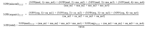
VVEG
VEMAP Vegetation Type
Küchler Vegetation Types

vveg.v1
vveg.v2
1
Tundra
52
52
2
Boreal coniferous forest
15, 21, 93, 96
15, 21, 93, 96
3
Temperate maritime coniferous forest
1, 2, 3, 4, 5, 6
1, 2, 3, 4, 5, 6
4
Temperate continental coniferous forest
8, 10, 11, 12, 13, 14, 16, 17, 18, 19, 20, 95
8, 10, 11, 12, 13, 14, 16, 17, 18, 19, 20, 95
5
Cool temperate mixed forest
28, 106, 107, 108, 109, 110
106, 107, 108, 109, 110
6
Warm temperate/ subtropical mixed forest
29, 89, 90, 111, 112
26, 28, 29, 89, 90, 111, 112
7
Temperate deciduous forest
26, 98, 99, 100, 101, 102, 103, 104
98, 99, 100, 101, 102, 103, 104
8
Tropical deciduous forest
not present
not present
9
Tropical evergreen forest
not present
not present
10
Temperate mixed xeromorphic woodland
30, 31, 32, 36, 37
30, 31, 32, 36, 37
11
Temperate conifer xeromorphic woodland
23
23
12
Tropical thorn woodland
not present
not present
13
(v1) Temperate/subtropical deciduous savanna
61, 71, 81, 82, 84, 87, 88
71, 81, 82, 84, 88

(v2) Temperate deciduous savanna

14
Warm temperate/ subtropical mixed savanna
60, 62, 83, 85, 86
60, 61, 62, 83, 85, 86, 87
15
Temperate conifer savanna
24
24
16
Tropical deciduous savanna
not present
not present
17
C3 grasslands
47, 48, 50, 51, 63, 64, 66, 67, 68
47, 48, 50, 51, 63, 64, 66, 67, 68
18
C4 grasslands
53, 54, 65, 69, 70, 74, 75, 76, 77
53, 54, 65, 69, 70, 74, 75, 76, 77
19
Mediterranean shrubland
33, 34, 35
33, 34, 35
20
Temperate arid shrubland
38, 39, 40, 46, 55, 56, 57
38, 39, 40, 46, 55, 56, 57
21
Subtropical arid shrubland
41, 42, 43, 44, 45, 58, 59
41, 42, 43, 44, 45, 58, 59
90
Ice
not present
not present
91
Inland water bodies
no symbol
no symbol
92
Wetlands
49, 78, 79, 80, 92, 94, 113, 114
49, 78, 79, 80, 92, 94, 113, 114
Table A3.2 Küchler Vegetation Type Names and Identifying Codes
(Küchler 1964, 1975).

Code
Küchler Vegetation Type
WESTERN FORESTS

Needleleaf Forests
1
Spruce-cedar hemlock forest
2
Cedar-hemlock-Douglas fir forest
3
Silver fir-Douglas fir forest
4
Fir-hemlock forest
5
Mixed conifer forest
6
Redwood forest
7
Red fir forest
8
Lodgepole pine-subalpine forest
9
Pine-cypress forest
10
Ponderosa shrub forest
11
Western ponderosa forest
12
Douglas fir forest
13
Cedar-hemlock-pine forest
14
Grand fir-Douglas fir forest
15
Western spruce-fir forest
16
Eastern ponderosa forest
17
Black Hills pine forest
18
Pine-Douglas fir forest
19
Arizona pine forest
20
Spruce-fir-Douglas fir forest
21
Southwestern spruce-fir forest
22
Great Basin pine forest
23
Juniper-pinyon woodland
24
Juniper steppe woodland

Broadleaf forests
25
Alder-ash forest
26
Oregon oakwoods
27
Mesquite bosques

Broadleaf and needleleaf forests
28
Mosaic of numbers 2 and 26
29
California mixed evergreen forest
30
California oakwoods
31
Oak-juniper woodland
32
Transition between 31 and 37

WESTERN SHRUB AND GRASSLAND

Shrub

33
Chaparral
34
Montane chaparral
35
Coastal sagebrush
36
Mosaic of numbers 30 and 35
37
Mountain mahogany-oak scrub
38
Great Basin sagebrush
39
Blackbrush
40
Saltbush-greasewood
41
Creosote bush
42
Creosote bush-bur sage
43
Palo verde-cactus shrub
44
Creosote bush-tarbush
45
Ceniza shrub
46
Desert: vegetation largely absent

Grasslands

47
Fescue-oatgrass
48
California steppe
49
Tule marshes
50
Fescue-wheatgrass
51
Wheatgrass-bluegrass
52
Alpine meadows and barren
53
Grama-galleta steppe
54
Grama-tobosa prairie

Shrub and grasslands combinations
55
Sagebrush steppe
56
Wheatgrass-needlegrass shrubsteppe
57
Galleta-three awn shrubsteppe
58
Grama-tobosa shrubsteppe
59
Trans-Pecos shrub savanna
60
Mesquite savanna
61
Mesquite-acacia savanna
62
Mesquite-live oak savanna

CENTRAL AND EASTERN GRASSLANDS

Grasslands

63
Foothills prairie
64
Grama-needlegrass-wheatgrass
65
Grama-buffalo grass
66
Wheatgrass-needlegrass
67
Wheatgrass-bluestem-needlegrass
68
Wheatgrass-grama-buffalo grass
69
Bluestem-grama prairie
70
Sandsage-bluestem prairie
71
Shinnery
72
Sea oats prairie
73
Northern cordgrass prairie
74
Bluestem prairie
75
Nebraska Sandhills prairie
76
Blackland prairie
77
Bluestem-sacahuista prairie
78
Southern cordgrass prairie
79
Palmetto prairie

Grassland and forest combinations
80
Marl-Everglades
81
Oak savanna
82
Mosaic of numbers 74 and 100
83
Cedar glades
84
Cross timbers
85
Mesquite-buffalo grass
86
Juniper-oak savanna
87
Mesquite-oak savanna
88
Fayette prairie
89
Blackbelt
90
Live oak-sea oats
91
Cypress savanna
92
Everglades

EASTERN FORESTS

Needleleaf forests
93
Great Lakes spruce-fir forest
94
Conifer bog
95
Great Lakes pine forest
96
Northeastern spruce-fir forest

Broadleaf forests
98
Northern floodplain forest
99
Maple-basswood forest
100
Oak-hickory forest
101
Elm-ash forest
102
Beech-maple forest
103
Mixed mesophytic forest
104
Appalachian oak forest
105
Mangrove

Broadleaf and needleleaf forests
106
Northern hardwoods
107
Northern hardwoods-fir forest
108
Northern hardwoods-spruce forest
109
Transition between numbers 104 and 106
110
Northeastern oak-pine forest
111
Oak-hickory-pine forest
112
Southern mixed forest
113
Southern floodplain forest
114
Pocosin
115
Sand pine scrub
116
Subtropical pine forest

A4 APPENDIX 4: STATE IDENTIFICATION NUMBERS

State identification codes used in the site files (Section 12) are:

1 Alabama
2 Arizona
3 Arkansas
4 California
5 Colorado
6 Connecticut
7 Delaware
8 Florida
9 Georgia
10 Idaho
11 Illinois
12 Indiana
13 Iowa
14 Kansas
15 Kentucky
16 Louisiana
17 Maine
18 Maryland
19 Massachusetts
20 Michigan
21 Minnesota
22 Mississippi
23 Missouri
24 Montana
25 Nebraska
26 Nevada
27 New Hampshire
28 New Jersey
29 New Mexico
30 New York
31 North Carolina
32 North Dakota
33 Ohio
34 Oklahoma
35 Oregon
36 Pennsylvania
37 Rhode Island
38 South Carolina
39 South Dakota
40 Tennessee
41 Texas
42 Utah
43 Vermont
44 Virginia
45 Washington
46 West Virginia
47 Wisconsin
48 Wyoming
49 unassigned
50 Alaska

[1] J.M. Melillo (Chair), J. Borchers, J. Chaney, A. Haxeltine, D.W. Kicklighter, A.D. McGuire, R. McKeown, R.P. Neilson, R.R. Nemani, D.S. Ojima, Y. Pan, W.J. Parton, L.L. Pierce, I.C. Prentice, W.M. Pulliam, B. Rizzo, S.W. Running, S. Sitch, T.M. Smith, and F.I. Woodward.

Category	File Structure	File Format	Access
Georeferencing	Gridded data	SVF*	CDROM, www, FTP
Monthly Climate	Gridded data	SVF	CDROM, www, FTP
Daily Climate	Sequential data	IEEE Binary	CDROM, www, FTP
Soil	Gridded data	SVF	CDROM, www, FTP
Vegetation	Gridded data	SVF	CDROM, www, FTP
Climate Scenarios	Gridded data	SVF	CDROM, www, FTP
Site	Sequential data	ASCII Columnar	CDROM, www, FTP
Bulk Transfer	Multiple files	UNIX Tarfiles	www, FTP
Phase I Model Results	Gridded data	SVF	www, FTP

Grid Position	Longitude*	Latitude
Lower Left Corner	-124.5deg.	25.0deg.
Upper Right Corner	-67.0deg.	49.0deg.

	Column
		1		-to-			115
Row 1		1	2	3	4	...	115
		116	117	118	119	...	230
		231	...
-to-		.
		.
		.
48						...	5520

Variable	Variable Type	Variable Width (columns)	Column Start	Column End	Scaling Factor
Grid Cell ID	numeric	4	1	4	1
Latitude	numeric	4	7	10	100
Longitude	numeric	5	12	16	-100
Elevation	numeric	4	19	22	1
vveg2 Vegetation Code	numeric	2	27	28	1
Küchler Vegetation Code	numeric	3	32	34	1
State ID	numeric	2	39	40	1
12 Monthly Values	numeric	6	41	112	(*)

Cell Type	Count
Non-background grid cells (including wetlands)	3261
Background cells (-9999)	2259
Total	5520

Cell Type	Count
Non-background grid cells (excluding wetlands)	3168
Background cells (-9999) (with wetland cells set to -9999)	2352
Total	5520

Variable Name Code	Description
elev	Average grid cell elevation
lat	Latitude of grid cell center
lon	Longitude of grid cell center
area	Absolute area of a grid cell
areap	Percent of a grid cell covered by land and within U.S. borders
varea	Absolute area of a grid cell covered by land and within U.S. borders

VAR	=	Variable name
elev		elevation [m]
lat		latitude [degrees and decimal degrees]
lon		longitude [degrees and decimal degrees]
area		absolute area [km²]
areap		percent VEMAP domain area [%]
varea		absolute VEMAP domain area [km²]

Variable Name Code	Description
tx, tn, tm	Maximum, minimum, mean temperature
r_atmax, r_atmin	Record absolute maximum, minimum temperature
r_mtmax, r_mtmin	Month of occurrence of record absolute maximum, minimum temperature
c_atmax, c_atmin	Characteristic year absolute maximum, minimum temperature
c_mtmax, c_mtmin	Month of occurrence of characteristic year absolute maximum, minimum temperature
p	Accumulated precipitation
sr	Total incident solar radiation at surface
fsr	'sr' as fraction potential total solar radiation at top of atmosphere (total atmospheric transmissivity: clear sky + cloud effects)
fsr_sfc	'sr' as fraction potential total solar radiation at surface (cloud transmissivity)
psr	Potential total solar radiation at top of atmosphere
psr_sfc	Potential total solar radiation at surface
irr	Mean daily irradiance
vp	Vapor pressure
rh	Relative humidity (mean for daylight hours)
w	Wind speed

VAR or VAR_sfc	=	Variable name
tx		maximum temperature [deg.C]
tn		minimum temperature [deg.C]
tm		mean temperature [deg.C]
p		precipitation [mm]
sr		total incident solar radiation [kJ/m²]
fsr		'sr' as fraction potential total solar radiation at top of atmosphere [0-1]
fsr_sfc		'sr' as fraction potential total solar radiation at surface [0-1]
psr		potential total solar radiation at top of atmosphere [kJ/m²]
psr_sfc		potential total solar radiation at surface [kJ/m²]
irr		mean irradiance [W/m²]
vp		vapor pressure [mb]
rh		mean daylight relative humidity [%]
w		wind speed [m/s]

.MMM	=	Period month (jan, feb, etc.) or annual (ann)

P_	=	Period
r		20-year WGEN record
c		characteristic year

VAR	=	Variable
atmax		absolute maximum temperature
atmin		absolute minimum temperature
mtmax		month of occurrence of absolute maximum temperature (e.g., 7 = July)
mtmin		month of occurrence of absolute minimum temperature (e.g., 1 = January)

Variable Name Code	*Layers (L)**	Description
modes	--	Number of modal soil profiles per cell
map	--	Percent areal coverage of mineral soil component within a modal or average soil (Corresponding variable for organic soil component is not included; 1 - map)
tap	--	Percent areal coverage of a given modal soil (or average soil) within the VEMAP land area of a grid cell
ma, oa	--	Absolute areal coverage of mineral (or organic) soil component within a modal or average soil
mbd	1, 2	Bulk density
mz, oz	--	Soil depth
msa, msi, mcl, moc	1, 2**	Texture: % sand, silt, clay, organic content
mrf, orf	1, 2	Rock fragments
mwh, owh	1, 2	Water holding capacity
tsoc, tsoc20	(0-100 cm, 0-20 cm)	Soil organic carbon

C	=	Soil component type
m		mineral soil
o		organic soil
t		total (both components combined)

VAR	=	Variable name
Mineral soils only (C = m)
ap		areal coverage of mineral soil [% of modal soil area]
sa		sand content of mineral soil [% by weight]
si		silt content of mineral soil [% by weight]
cl		clay content of mineral soil [% by weight]
bd		bulk density of mineral soil [g/cm³]
oc		organic content of mineral soil [% by weight]

Mineral and organic soils (C = m, o)
wh		water holding capacity [cm H₂O]
z		depth [cm]
a		area [km²]
rf		rock fragments [% by volume]

Total (C = t; omitted for modes)
modes		number of modal soil profiles per cell
tap		mode area [% of cell land area]
tsoc		soil organic carbon (0-100 cm) [mg C/ha]
tsoc20		soil organic carbon (0-20 cm) [mg C/ha]

L	=	Layer
1		0 - 50 cm
2		50 - 150 cm

_mM or .mM	=	Modal soil profile id# (M = 1 to 4, with m1 representing the most dominant profile
_ave or .ave	=	Average soil profile

Variable Name Code	Description
vveg	Current distribution of VEMAP vegetation class

vveg Code	Vegetation Type
TUNDRA
1	Tundra
FOREST
2	Boreal Coniferous Forest
	(includes Boreal/Temperate Transitional and Temperate Subalpine Forests)
3	Maritime Temperate Coniferous Forest
4	Continental Temperate Coniferous Forest
5	Cool Temperate Mixed Forest
6	Warm Temperate/Subtropical Mixed Forest
7	Temperate Deciduous Forest
8	Tropical Deciduous Forest (not present)**
9	Tropical Evergreen Forest (not present)
XEROMORPHIC WOODLANDS and FORESTS
10	Temperate Mixed Xeromorphic Woodland
11	Temperate Conifer Xeromorphic Woodland
12	Tropical Thorn Woodland (not present)
SAVANNAS
13	Temperate/Subtropical Deciduous Savanna (.v1)
	Temperate Deciduous Savanna (.v2)
14	Warm Temperate / Subtropical Mixed Savanna
15	Temperate Conifer Savanna
16	Tropical Deciduous Savanna (not present)
GRASSLANDS
17	C3 Grasslands (includes Short, Mid-, and Tall C3 Grasslands)
18	C4 Grasslands (includes Short, Mid-, and Tall C4 Grasslands)

SHRUBLANDS
19	Mediterranean Shrubland
20	Temperate Arid Shrubland
21	Subtropical Arid Shrubland
EXCLUDED SURFACE TYPES
90	Ice (not present)
91	Inland Water Bodies (includes ocean inlets)
92	Wetlands (includes floodplains and strands)

		Climate Scenario
Variable Name	Change Field Type	CCC	GFDL R15 Q-flux	GFDL R15	GFDL R30	GISS	RegCM	OSU	UKMO
tx	diff						X
tn	diff						X
t, tm	diff	X	X	X	X	X	X	X	X
rh	diff		X	X	X	X		X	X
p	ratio	X	X	X	X	X	X	X	X
sr	ratio	X	X	X	X	X	X	X	X
vp	ratio		X	X	X	X	X	X	X
w	ratio	X	X	X	X	X	X	X	X

VAR	=	Variable name
t, tm		surface air mean temperature difference (2xCO₂-1xCO₂)
tx, tn		surface air maximum or minimum temperature difference (2xCO₂-1xCO₂)
rh		relative humidity difference (2xCO₂-1xCO₂)
p		precipitation change ratio (2xCO₂/1xCO₂)
sr		total incident solar radiation change ratio (2xCO₂/1xCO₂)
vp		surface vapor pressure change ratio (2xCO₂/1xCO₂)
w		surface wind speed change ratio (2xCO₂/1xCO₂)

_GGG	=	Climate model experiment
ccc		CCC
gf1		GFDL R15
gfq		GFDL R15 Q-flux
gf3		GFDL R30
gis		GISS
mm4		RegCM (MM4)
osu		OSU
ukm		UKMO

.MMM	=	Period month (e.g., jan, feb) or annual (ann)

VVEG	VEMAP Vegetation Type	Küchler Vegetation Types
		vveg.v1	vveg.v2
1	Tundra	52	52
2	Boreal coniferous forest	15, 21, 93, 96	15, 21, 93, 96
3	Temperate maritime coniferous forest	1, 2, 3, 4, 5, 6	1, 2, 3, 4, 5, 6
4	Temperate continental coniferous forest	8, 10, 11, 12, 13, 14, 16, 17, 18, 19, 20, 95	8, 10, 11, 12, 13, 14, 16, 17, 18, 19, 20, 95
5	Cool temperate mixed forest	28, 106, 107, 108, 109, 110	106, 107, 108, 109, 110
6	Warm temperate/ subtropical mixed forest	29, 89, 90, 111, 112	26, 28, 29, 89, 90, 111, 112
7	Temperate deciduous forest	26, 98, 99, 100, 101, 102, 103, 104	98, 99, 100, 101, 102, 103, 104
8	Tropical deciduous forest	not present	not present
9	Tropical evergreen forest	not present	not present
10	Temperate mixed xeromorphic woodland	30, 31, 32, 36, 37	30, 31, 32, 36, 37
11	Temperate conifer xeromorphic woodland	23	23
12	Tropical thorn woodland	not present	not present
13	(v1) Temperate/subtropical deciduous savanna	61, 71, 81, 82, 84, 87, 88	71, 81, 82, 84, 88
	(v2) Temperate deciduous savanna
14	Warm temperate/ subtropical mixed savanna	60, 62, 83, 85, 86	60, 61, 62, 83, 85, 86, 87
15	Temperate conifer savanna	24	24
16	Tropical deciduous savanna	not present	not present
17	C3 grasslands	47, 48, 50, 51, 63, 64, 66, 67, 68	47, 48, 50, 51, 63, 64, 66, 67, 68
18	C4 grasslands	53, 54, 65, 69, 70, 74, 75, 76, 77	53, 54, 65, 69, 70, 74, 75, 76, 77
19	Mediterranean shrubland	33, 34, 35	33, 34, 35
20	Temperate arid shrubland	38, 39, 40, 46, 55, 56, 57	38, 39, 40, 46, 55, 56, 57
21	Subtropical arid shrubland	41, 42, 43, 44, 45, 58, 59	41, 42, 43, 44, 45, 58, 59
90	Ice	not present	not present
91	Inland water bodies	no symbol	no symbol
92	Wetlands	49, 78, 79, 80, 92, 94, 113, 114	49, 78, 79, 80, 92, 94, 113, 114

Code	Küchler Vegetation Type
WESTERN FORESTS

Needleleaf Forests
1	Spruce-cedar hemlock forest
2	Cedar-hemlock-Douglas fir forest
3	Silver fir-Douglas fir forest
4	Fir-hemlock forest
5	Mixed conifer forest
6	Redwood forest
7	Red fir forest
8	Lodgepole pine-subalpine forest
9	Pine-cypress forest
10	Ponderosa shrub forest
11	Western ponderosa forest
12	Douglas fir forest
13	Cedar-hemlock-pine forest
14	Grand fir-Douglas fir forest
15	Western spruce-fir forest
16	Eastern ponderosa forest
17	Black Hills pine forest
18	Pine-Douglas fir forest
19	Arizona pine forest
20	Spruce-fir-Douglas fir forest
21	Southwestern spruce-fir forest
22	Great Basin pine forest
23	Juniper-pinyon woodland
24	Juniper steppe woodland

Broadleaf forests
25	Alder-ash forest
26	Oregon oakwoods
27	Mesquite bosques

Broadleaf and needleleaf forests
28	Mosaic of numbers 2 and 26
29	California mixed evergreen forest
30	California oakwoods
31	Oak-juniper woodland
32	Transition between 31 and 37

WESTERN SHRUB AND GRASSLAND

Shrub
33	Chaparral
34	Montane chaparral
35	Coastal sagebrush
36	Mosaic of numbers 30 and 35
37	Mountain mahogany-oak scrub
38	Great Basin sagebrush
39	Blackbrush
40	Saltbush-greasewood
41	Creosote bush
42	Creosote bush-bur sage
43	Palo verde-cactus shrub
44	Creosote bush-tarbush
45	Ceniza shrub
46	Desert: vegetation largely absent

Grasslands
47	Fescue-oatgrass
48	California steppe
49	Tule marshes
50	Fescue-wheatgrass
51	Wheatgrass-bluegrass
52	Alpine meadows and barren
53	Grama-galleta steppe
54	Grama-tobosa prairie

Shrub and grasslands combinations
55	Sagebrush steppe
56	Wheatgrass-needlegrass shrubsteppe
57	Galleta-three awn shrubsteppe
58	Grama-tobosa shrubsteppe
59	Trans-Pecos shrub savanna
60	Mesquite savanna
61	Mesquite-acacia savanna
62	Mesquite-live oak savanna

CENTRAL AND EASTERN GRASSLANDS

Grasslands
63	Foothills prairie
64	Grama-needlegrass-wheatgrass
65	Grama-buffalo grass
66	Wheatgrass-needlegrass
67	Wheatgrass-bluestem-needlegrass
68	Wheatgrass-grama-buffalo grass
69	Bluestem-grama prairie
70	Sandsage-bluestem prairie
71	Shinnery
72	Sea oats prairie
73	Northern cordgrass prairie
74	Bluestem prairie
75	Nebraska Sandhills prairie
76	Blackland prairie
77	Bluestem-sacahuista prairie
78	Southern cordgrass prairie
79	Palmetto prairie

Grassland and forest combinations
80	Marl-Everglades
81	Oak savanna
82	Mosaic of numbers 74 and 100
83	Cedar glades
84	Cross timbers
85	Mesquite-buffalo grass
86	Juniper-oak savanna
87	Mesquite-oak savanna
88	Fayette prairie
89	Blackbelt
90	Live oak-sea oats
91	Cypress savanna
92	Everglades

EASTERN FORESTS

Needleleaf forests
93	Great Lakes spruce-fir forest
94	Conifer bog
95	Great Lakes pine forest
96	Northeastern spruce-fir forest

Broadleaf forests
98	Northern floodplain forest
99	Maple-basswood forest
100	Oak-hickory forest
101	Elm-ash forest
102	Beech-maple forest
103	Mixed mesophytic forest
104	Appalachian oak forest
105	Mangrove

Broadleaf and needleleaf forests
106	Northern hardwoods
107	Northern hardwoods-fir forest
108	Northern hardwoods-spruce forest
109	Transition between numbers 104 and 106
110	Northeastern oak-pine forest
111	Oak-hickory-pine forest
112	Southern mixed forest
113	Southern floodplain forest
114	Pocosin
115	Sand pine scrub
116	Subtropical pine forest