Documentation Revision Date: 2020-09-30
Dataset Version: 1
Summary
Vulcan v3.0 is the first bottom-up inventory to report FFCO2 plus cement production CO2 fluxes at 1-km resolution for all major carbon-emitting sectors across the entire United States landscape. Vulcan v3.0 is constructed from numerous public datasets that generate the magnitude, spatial representation, and temporal representation of FFCO2 emissions.
There are 66 data files in standardized netCDF version 4 format associated with this dataset. This includes a set of 33 files for each of the two geographic areas: the contiguous United States and Alaska. Each file contains 6 time steps, one for each year in 2010 - 2015. For each sector, there are unique files representing the central estimate of annual total emissions, the upper 95% confidence interval boundary, and the lower 95% confidence interval boundary.
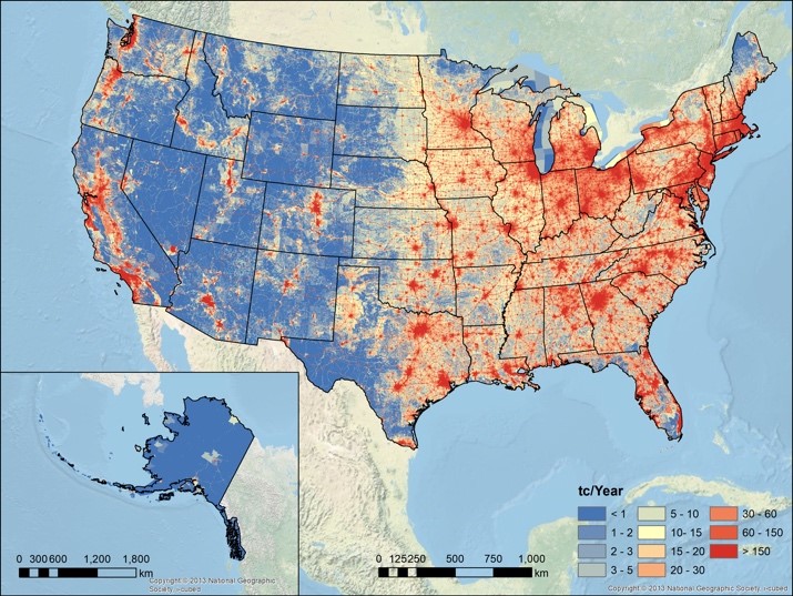
Figure 1. Vulcan v3.0 FFCO2 emissions (tC/km2/year) for the United States in year 2011 at 1-km resolution. Source: Figure 3(a) in Gurney et al., 2020.
Citation
Gurney, K.R., J. Liang, R. Patarasuk, Y. Song, J. Huang, and G. Roest. 2019. Vulcan: High-Resolution Annual Fossil Fuel CO2 Emissions in USA, 2010-2015, Version 3. ORNL DAAC, Oak Ridge, Tennessee, USA. https://doi.org/10.3334/ORNLDAAC/1741
Table of Contents
- Dataset Overview
- Data Characteristics
- Application and Derivation
- Quality Assessment
- Data Acquisition, Materials, and Methods
- Data Access
- References
Dataset Overview
The Vulcan version 3.0 annual dataset provides estimates of annual carbon dioxide (CO2) emissions from the combustion of fossil fuels (FF) and CO2 emissions from cement production for the conterminous United States and the State of Alaska. Referred to as FFCO2, the emissions from Vulcan are categorized into 10 source sectors including; residential, commercial, industrial, electricity production, onroad, nonroad, commercial marine vessel, airport, rail, and cement. Data are gridded annually on a 1-km grid for the years 2010 to 2015. These data are annual sums of hourly estimates. Also provided are estimates of the upper 95% confidence interval and the lower 95% confidence interval boundaries for each emission estimate. For each uncertainty level, there are 10 individual sector files and one total file. These data are designed to be used as emission estimates in atmospheric transport modeling, policy, mapping, and other data analyses and applications.
Vulcan v3.0 is the first bottom-up inventory to report FFCO2 plus cement production CO2 fluxes at 1-km resolution for all major carbon-emitting sectors across the entire United States landscape. Vulcan v3.0 is constructed from numerous public datasets that generate the magnitude, spatial representation, and temporal representation of FFCO2 emissions.
Project: North American Carbon Program
The North American Carbon Program (NACP) is a multidisciplinary research program designed to improve understanding of North America's carbon sources, sinks, and stocks. The central objective is to measure and understand the sources and sinks of Carbon Dioxide (CO2), Methane (CH4), and Carbon Monoxide (CO) in North America and adjacent oceans. The NACP is supported by a number of different federal agencies.
Related Publication:
Gurney, K. R., Liang, J., Patarasuk, R., Song, Y., Huang, J., & Roest, G. (2020). The Vulcan Version 3.0 High Resolution Fossil Fuel CO2 Emissions for the United States. Journal of Geophysical Research: Atmospheres, 125, e2020JD032974. https://doi.org/10.1029/2020JD032974
Related Dataset:
Gurney, K.R., J. Liang, R. Patarasuk, Y. Song, J. Huang, and G. Roest. 2020. Vulcan: High-Resolution Hourly Fossil Fuel CO2 Emissions in USA, 2010-2015, Version 3. ORNL DAAC, Oak Ridge, Tennessee, USA. https://doi.org/10.3334/ORNLDAAC/1810
Acknowledgements:
This research was supported primarily by the National Aeronautics and Space Administration grant NNX14AJ20G and the NASA Carbon Monitoring System program, Understanding User Needs for Carbon Information project (subcontract 1491755). Earlier versions of the Vulcan FFCO2+ emissions data product were supported by NASA grant Carbon/04-0325-0167 and DOE grant DE-AC02- 05CH11231.
Data Characteristics
Spatial Coverage: Two geographic regions: contiguous United States and the State of Alaska
Spatial Resolution: 1-km grid
Temporal Coverage: 2010-2015
Temporal Resolution: Annual
Study Areas (All latitude and longitude given in decimal degrees)
|
Site |
Westernmost Longitude | Easternmost Longitude | Northernmost Latitude | Southernmost Latitude |
|---|---|---|---|---|
| Contiguous USA | -128.22655 | -65.30824167 | 47.89015278 | 22.85824167 |
| Alaska | -165.2138056 | -127.1191611 | 73.75332778 | 39.75995278 |
Data File Information
There are 66 netCDF version 4 (*.nc4) data files provided with this dataset. This includes 33 files for each of the two geographic areas -- the Conterminous United States and Alaska.
These netCDF files contain parameter and spatial metadata within the file header following Climate and Forecast metadata convention version 1.6 (CF-1.6, https://cfconventions.org).
File organization
The 6 years of annual estimates, 2010-2015, are included in each *.nc4 file.
For each of the 10 source sectors and the total emissions, there are output files for (1) the central mean estimates, (2) the upper 95% confidence intervals, and (3) the lower 95% confidence interval boundaries. That is 11 emissions estimates x 3 output types for each geographic area = 33 files.
File naming conventions
Example file names:
Vulcan_v3_AK_annual_1km_airport_mn.nc4
Vulcan_v3_AK_annual_1km_airport_hi.nc4
Vulcan_v3_AK_annual_1km_airport_lo.nc4
File name syntax:
Vulcan_v3_<domain>_annual_1km_<sector>_<uncertainty>.nc4
domain: Alaska (_AK) or the contiguous US (_US).
sector: airport, cement, cmv, commercial, elec_prod, industrial, nonroad, onroad, railroad, residential, or total). See descriptions below.
uncertainty:
_mn for central estimate of annual total emissions,
_lo for the lower 95% confidence interval boundary value,
_hi for the upper 95% confidence interval boundary.
Data properties
Units are metric tonnes of carbon per gridcell (1 km2) per year (tC/km2/year).
Missing values are represented by -9999.
| Sector Code | Description |
|---|---|
| airport | Airport sector (taxi/takeoff to 3000’) |
| cement | Cement production sector |
| cmv | Commercial Marine Vessel sector |
| commercial | Commercial sector |
| elec_prod | Electricity production sector |
| industrial | Industrial sector |
| nonroad | Nonroad sector (e.g. snowmobiles, ATVs) |
| onroad | Onroad sector |
| railroad | Railroad sector |
| residential | Residential sector |
| total | Total emissions |
Coordinate reference system
Datum: WGS84
Projection: Lambert Conformal Conic (LCC)
Units: meter
False easting: 0.0 m
False northing: 0.0 m
Longitude of origin: -97.0°
Latitude of origin: 40.0°
Standard parallel 1: 33.0°
Standard parallel 2: 45.0°
Proj.4 string: +proj=lcc +lat_1=33 +lat_2=45 +lat_0=40 +lon_0=-97 +x_0=0 +y_0=0 +ellps=WGS84 +units=m +no_defs
Application and Derivation
The Vulcan v3.0 FFCO2 emissions data product can be applied to both scientific and policy-related objectives. It can supply a high-resolution boundary condition (“prior”) to atmospheric CO2 inverse efforts to better isolate biospheric net exchange or as a direct constraint to assessing anthropogenic fluxes. Better understanding both the FFCO2 emissions and the net biosphere carbon exchange improves projections of climate change through more reliable estimation of climate-carbon feedback. It can also be used in direct policymaking by offering more granular detail on FFCO2 emission processes and magnitudes. This can provide sub-national stakeholders with more optimal policy choices, isolating the timing and location of the largest-emit entities for more specific and targeted mitigation.
Quality Assessment
The uncertainty of the Vulcan results are estimated by attempting to capture key input parameter variation. This is accomplished by completing a simulation with key input parameters (e.g. CO emission factor, CO2 emission factor, CO emissions) set at their upper and lower range (an approximate 95% confidence interval). These two additional simulations estimated total annual domain FFCO2 emissions as -14.0%/+16.6% of the central estimate for the example year of 2011.
Two separate techniques are used to test the general quality of the Vulcan v3.0 FFCO2 emissions estimate. The first is a comparison to other similar space/time-resolved FFCO2 emission data products. Comparison to the ACES granular FFCO2 estimate which only covers 13 Northeastern states was performed. In this comparison, total relative difference of 1.7% (ACES>Vulcan) was found, but much larger differences at the grid cell scale with a grid cell absolute median relative difference of 53.4%. Vulcan v3.0 results were also compared to the ODIAC global gridded FFCO2 emissions data product which found a total relative difference of 6.9% (100.3 MtC/yr; Vulcan>ODIAC) in 2011. At the grid cell-scale a grid cell absolute median relative difference of 104.4% was observed. See Gurney et al. (2020) for more details.
A second approach that compared the results presented here to atmospheric CO2 inverse estimates was performed. At the whole contiguous US spatial scale and annual temporal scale, the 2010 Vulcan results were within 1.4% of an atmospheric 14CO2 inversion effort (Basu et al., 2020).
Data Acquisition, Materials, and Methods
Vulcan v3.0 is a bottom-up high-resolution model for FFCO2 and cement production CO2. Vulcan generates these FFCO2+ emissions for the years 2010 to 2015, annually on a 1 km x 1 km grid with sector-specific output.
Following are brief descriptions of the data sources and processing methods employed to create the Vulcan v3.0 emission products. A bibliography for the data sources is provided at the end of this section. For details and descriptions of uncertainty calculations please refer to Gurney et al. (2020).
Data Sources
Emissions of FFCO2 from the residential, commercial, industrial, nonroad, commercial marine vessels, airport, and rail sectors were derived from the CO emissions reporting within the U.S. Environmental Protection Agency’s (EPA) National Emissions Inventory (NEI) for 2011 (EPA, 2015a). Emissions from electricity production were derived from three datasets: the Environmental Protection Agency’s Clean Air Markets Division (CAMD) data (USEPA, 2015b); the Department of Energy’s Energy Information Administration (EIA) reporting data (DOE/EIA, 2003); reporting within the NEI point source reporting.
For onroad FFCO2 emissions, county scale results are retrieved from the 2011 EPA NEIv1 onroad output (USEPA, 2011), based on simulations using the Motor Vehicle Emissions Simulator (MOVES) model with inputs supplied to a county database (CDB) by SLT agencies (USEPA, 2012; USEPA, 2015a). The state of California did not report FFCO2 to the 2011 NEI. Hence, the Vulcan onroad FFCO2 emissions for California used the 2011 results from the Emissions FACtors 2014 model (EMFAC2014), produced by the California Air Resources Board (CARB, 2014).
CO2 emissions from cement production utilizes two datasets: the data provided by the Portland Cement Association which provides the annual clinker capacity at individual facilities (PCA, 2006); and the Minerals Yearbook produced by the United States Geological Survey (USGS 2013).
Distribution of the sources to space and time utilize numerous federal datasets outlined in Table 1. Further details are provided in the following methods sub-sections.
Table 1. Data sources used to derive the Vulcan v3.0 FFCO2 emissions data product. A bibliography for the sources is provided at the end of this section.
| Sector/type | Emissions Data Source | Original spatial resolution/information | Spatial distribution | Temporal distribution |
|---|---|---|---|---|
| Onroad | EMFAC a CO2, EPA NEIb onroad CO2 | County, road class, vehicle class | FHWA AADTc | CCSe |
| Electricity production | CAMDf CO2, DOE/EIAg fuel, EPA NEI point CO | Lat/lon, fuel type, technology | EPA/EIA NEI Lat/Lon, Google Earth | CAMD, EIA and EPA |
| Residential nonpoint buildings | EPA NEI nonpoint CO | County, fuel type | FEMA HAZUSd, DOE RECS NE-EUIh | eQUESTi model |
| Nonroad | NEI nonpoint CO | County, vehicle class | EPA spatial surrogates (vehicle class specific) | EPA temporal surrogates (by SCCj) |
| Airport | EPA NEI point CO | Lat/lon, aircraft class | Lat/Lon | LAWA & OPSNETk |
| Commercial nonpoint buildings | EPA NEI nonpoint CO | County, fuel | FEMA HAZUS, DOE CBECS NE-EUIl | eQUEST model |
| Commercial point sources | EPA NEI point CO | Lat/lon, fuel type, combustion technology | EPA NEI Lat/Lon, Google Earth | eQUEST model |
| Industrial point sources | EPA NEI point CO | Lat/Lon, fuel type, combustion technology | EPA NEI Lat/Lon, Google Earth | EPA temporal surrogates (by SCC) |
| Industrial nonpoint buildings | EPA NEI nonpoint CO | County, fuel type | FEMA HAZUS, DOE MECS NE-EUIm | eQUEST model |
| Commercial Marine Vessels | EPA NEI nonpoint CO | County, fuel type, port/underway | EPA port and shipping lane shapefiles | Flat time structure |
| Railroad | EPA NEI nonpoint CO, EPA NEI point CO | County, fuel type, segment | EPA NEI rail shapefile and density distribution | Pointwise records: EPA temporal surrogates (by SCC), nonpoint: flat time structure |
| Cement | Portland Cement Association, USGS | Lat/lon | PCA lat/lon checked in Google Earth | Flat time structure |
Footnotes:
a. Emissions Factors Model
b. Environmental Protection Agency, National Emissions Inventory
c. Federal Highway Administration, Annual Average Daily Traffic
d. Federal Emergency Management Agency
e. Continuous Count Stations
f. Clean Air Markets Division
g. Department of Energy/Energy Information Administration
h. Department of Energy Residential Energy Consumption Survey, non-electric energy use intensity
i. Quick Energy Simulation Tool
j. Source Classification Code
k. Los Angeles World Airport, The Operations Network
l. Department of Energy Commercial Energy Consumption Survey, non-electric energy use intensity
m. Department of Energy Manufacturing Energy Consumption Survey, non-electric energy use intensity
Methods
[Note that equations given in Gurney et al. (2020) have been omitted to simplify presentation of the following text.]
Nonpoint source (residential, commercial, industrial)
Fossil fuel CO2 emissions are created from NEI-reported county-scale CO reporting through the application of CO and CO2 emission factors. Where the CO2 emissions for a process n (e.g. industrial 10 MMBTU boiler, industrial gasoline reciprocating turbine) and fuel f (e.g. natural gas, bituminous coal); are the equivalent amount of CO emissions for a process n and fuel f; is the CO emission factor for a process n and fuel f; and is the CO2 EF for a process n and fuel f. The CO EF is retrieved from two categories of source information: 1) “self-reported” values (supplied by state or federal air quality specialists submitting the CO emissions reporting: ftp://newftp.epa.gov/air/nei/2011/doc/2011v2_supportingdata/nonpoint/) or 2) “default” values generated from a combination of values retrieved from the EPA WebFIRE EF database (https://cfpub.epa.gov/webfire/) and values accumulated through literature review. The self-reported CO EF values are assessed for reliability and replaced by a default value if the self-reported value is less than 0.1 or greater than 5 times the identified default value.
The state total FFCO2 emissions calculated as described above are compared to sector and fuel-specific fuel consumption totals reported by the Department of Energy/Energy Information Administration (DOE/EIA) State Energy Data System (DOE/EIA, 2018). Adjustment of the Vulcan state/sector/fuel totals are made to the nonpoint residential and commercial sectors only and for natural gas and petroleum fuel (aggregate) only.
Sub-county distribution of the county/sector/fuel-specific FFCO2 emissions to US Census block-groups uses the total floor area (m2) of buildings (specific to a building class) within each US Census block-group combined with estimates of energy use intensity (EUI). The general approach follows: where the total emissions, TE, associated with a building of type, n, using fuel, f, in a block-group, bg, is equal to the product of the total floor area, TFA, and the energy use intensity, EUI, of buildings in a census division, cd.
Building floor area is retrieved from HAZUS General Building Stock data collected and compiled by the Federal Emergency Management Agency (FEMA, 2017). The non-electric energy use intensity (NE-EUI; joules/m2) values are compiled by the DOE from building consumption energy surveys in different regions of the US (CBECS, 2016; MECS, 2010; RECS, 2013).
The product of the total building area for a given Census block-group/sector/building type combination and the sector/building type/fuel NE-EUI values act as a distributional fraction of the county total county/sector/fuel FFCO2 to each Census block-group. Hence this acts to provide a relative distribution of building FFCO2 emission within a US county only.
The time distribution of the annual FFCO2 emissions for the nonpoint data source uses a building energy model, eQuest, to generate simulated building energy consumption which, in turn, is used to represent hourly time patterns (Hirsch & Associates, 2004).
Point sources (commercial, industrial)
Each point emission record is also associated with an SCC which is used to retrieve the needed CO and CO2 EFs to enact the same procedure outlined in the description of the nonpoint source processing. All point source emission records designated as industrial, railroad, and nonroad are distributed to hourly temporal resolution from the 2011 annual total using SCC-specific temporal surrogate profiles provided by the EPAs Clearinghouse for Inventories and Emissions Factors (CHIEF) (USEPA, 2015c). The temporal surrogate profiles are constructed from monthly, weekly and diurnal cycles (data available at: ftp://newftp.epa.gov/air/emismod/2011/v3platform/ancillary_data/ge_dat_for_2011v3_temporal.zip). These temporal surrogates are comprised of three cyclic time profiles (diurnal, weekly, monthly) specific to SCC that are combined to generate hourly SCC-specific time fractions for an entire calendar year. Records which do not have an SCC match are distributed as a constant hourly emission.
Electricity production
Overlap exists between these three data sources (described above) which is corrected according to the prioritization in the order listed above. A detailed comparison made between the CAMD and EIA FFCO2 emissions along with greater detail regarding data sources, data processing and procedures can be found in Gurney et al. (2016).
Some manual corrections are performed to the geocoordinates of both the CAMD and EIA electricity production data, as a result of searching in Google Earth or via alternative online information resources (e.g. utility websites).
A hierarchy was employed given that there was overlap between the two datasets. This was performed at the unit level given that a single facility might have individual power units reporting to CAMD and another only reporting to the EIA. Where overlap did exist at this scale, preference was made to retain the CAMD data. Further details and rationale can be found in Gurney et al. (2016).
Onroad
County-scale FFCO2 emissions for all US states are spatially assigned to road segments via a road basemap that best represents the entirety of the road surface occupied by onroad vehicles. Vulcan uses a combination of the 2011 Highway Performance Monitoring System (HPMS, 2017) road network and Open Street Map (OSM; http://download.geofabrik.de/) road network. The Census Urbanized Areas boundary (https://www.fhwa.dot.gov/policyinformation/hpms/shapefiles.cfm) was used to assign an urban/rural distinction to each of the 7 original HPMS road classes making them compatible with the onroad NEI road classes (supplementary material, Table S4).
The distribution of the county-scale road/vehicle-specific FFCO2 emissions along the complete length of road class in a county, is achieved through the use of the 2011 AADT data from the FHWA’s HPMS (http://www.fhwa.dot.gov/policyinformation/hpms/shapefiles.cfm; state scale data files were used).
With a complete US map of AADT values and road segment length, the vehicle miles traveled (VMT) can be estimated. The fraction of a non-local road class-specific road segment’s VMT within a county acts as the distribution means to allocate county-scale onroad FFCO2. For local roads, given the paucity of AADT data, the fraction of a road segment’s length out of all local roads within a county acts as the allocation method.
Hourly traffic volume data for the years 2011-2013 were obtained from the FHWA Continuous Count Stations (CCS) dataset (previously known as the Automatic Traffic Recorder; ATR) (Jessberger, 2016). The CCS stations measure hourly traffic volume at a fixed location in space and we use the station’s latitude and longitude as a unique station identifier.
In order to distribute the temporal distribution measured at the gap-filled CCS measurement stations to all road segments in the US, interpolation/extrapolation of the traffic patterns is required. Given the paucity of traffic measurement stations relative to the total area of the US landscape and the fact that the temporal distribution of traffic is less related to road class than space, it was determined to aggregate the eight road classes to four, “temporal” road classes for purposes of spatial interpolation.
Inverse Distance Weighted (IDW) interpolation was performed for each of the four temporal road classes separately, and only for grid cells that are occupied by roads of that road class. The two inputs are the gap-filled CCS traffic data, and the locations of road segments for each of the four road classes.
Nonroad
The results used here are based on output from the National Mobile Inventory Model (NMIM) which relies on data inputs from the National County Data base (NCD) (USEPA 2005c; 2005d). Both the NMIM and the NCD were described previously (Gurney et al., 2009). The EPA updated data within the NCD from 12 SLT agencies along with EPA default values to generate the results in the 2011 NEIv2 (for a description of these updates see ftp://ftp.epa.give/EmisInventory/2011/doc/2011neiv2_supdata_nonroad).
As with the onroad sector, California presents a special case. The CO emissions are reported comprehensively using California’s OFFROAD model (www.arb.ca.gov/msei/offroad/offroad.htm ) but no CO2 was reported. Hence, we scaled the California CO emissions by the mean SCC-specific CO2/CO ratio from all other US counties.
Spatial distribution uses the spatial surrogates generated by the EPA reflecting a series of spatial representations such as the mines, golf course and agricultural land (The shapefiles can be found here: ftp://ftp.epa.gov/EmisInventory/emiss_shp2003/us/ or ftp://ftp.epa.gov/EmisInventory/2011v6/v1platform/spatial_surrogates/shapefiles/). There were instances in which nonroad FFCO2 emissions could not be associated with a spatial entity due to missing data. These emissions are spatialized by first aggregating all the unassociated sub-county emission elements to the county scale for a given spatial shape (e.g., golf courses, mines) and then distributing these emissions evenly across the county.
The sub-annual temporal distribution of the nonroad FFCO2 emissions uses SCC-specific temporal surrogate profiles provided by the EPAs Clearinghouse for Inventories and Emissions Factors (CHIEF) (USEPA, 2015c). The temporal surrogate profiles are constructed from monthly, weekly and diurnal cycles (data available at: ftp://newftp.epa.gov/air/emismod/2011/v3platform/ancillary_data/ge_dat_for_2011v3_temporal.zip). These temporal surrogates are comprised of three cyclic time profiles (diurnal, weekly, monthly) specific to SCC that are combined to generate hourly SCC-specific time fractions for an entire calendar year.
Airport
The airport FFCO2 emissions are only associated with the taxi & takeoff/landing sequences. The airports are geocoded to the airport location in the NEI though some manual adjustments have been made to the original coordinates using manual inspection in Google Earth.
Temporal distribution of the FFCO2 airport emissions use a series of datasets. The Los Angeles World Airports (LAWA) dataset reports hourly flight volume for three airports in the LA Basin domain: Los Angeles International airport (LAX), Ontario airport (ONT), and Van Nuys airport (VNY) (Hastings, 2014). The Operations Network (OPSNET) dataset from the FAA reports total date-specific, daily flight volume (365 values) at specific airports (https://aspm.faa.gov/opsnet/sys/Default.asp). An hourly time profile was constructed by combining the LAWA diurnal profile and the OPSNET annual profile. The three LAWA airports constituted the diurnal cycle at all US airports with the LAX assigned to international airports, the ONT to non-international airports and the VNY to local airports.
Airports were matched with a Federal Aviation Administration (FAA) international airport database (FAAINTL) by airport code to determine whether an airport is international (https://hub.arcgis.com/datasets/4782d6f5aa844591a16d46df635b7af4_1). Airports which could not be matched to the OPSNET data by airport code/airport name were assigned a temporal invariant (“flat”) hourly time structure.
Railroad
The 2011 NEIv2 CO emissions reporting results were originally developed for the 2008 NEI (ERG 2011) and scaled to 2011 values (ERG 2012). Emissions related to the railroad sector were reported as a mixture of nonpoint and point emissions and hence, these were managed separately but combined when represented as spatial entities. The CO emissions were converted to FFCO2 following the procedures outlined in the nonpoint and the point sections, respectively. The point source railroad emissions are associated with rail yards and related geo-specific locales and are placed in space according to the provided latitude and longitude. The railroad FFCO2 emissions associated with the nonpoint NEI reporting contain an ID variable that links to a spatial element (rail line segment) in the EPA railroad GIS shapefile (https://www.epa.gov/sites/production/files/2015-06/railway_20140730.zip). A large number of railroad emission records have no railroad segment match and are spatialized using freight statistics described in supplementary material. The annual railroad FFCO2 emissions are distributed to the hourly timescale with no additional temporal structure (a “flat” time distribution), unless they originated from point source data for which the SCC-specific time profiles, previously described, are used.
Commercial Marine Vessels (CMV)
The CMV emissions encompass maneuvering, hoteling, cruise and reduced speed zone travel and are specific to geographically located ports and shipping lanes that extend 12 nautical miles from the US shoreline. As with the nonroad reporting, the EPA used a mixture of SLT data submissions and default values, in collaboration with the Office of Transportation and Air Quality to generate an estimate of CO emissions for CMV. The spatialization utilized the EPA shapefiles that delineate US ports and US shipping lanes through spatial IDs associated with the emission records (https://www.epa.gov/sites/production/files/2015-06/ports_20140729.zip; https://www.epa.gov/sites/production/files/2015-06/shippinglanes_072914.zip). In the instance that no spatial entity is identified for an emission record, a simple spatial alternative is employed whereby all the unlinked port (or “underway”) emissions are summed within a county and evenly distributed to the shapes that are identified within that county (either ports or shipping lanes).
The CMV sector has no data allowing for the designation of hourly time structure. Hence, the emissions are temporally invariant over all hours of the year (“flat” distribution).
Cement
The geolocation for each of the individual facilities was achieved by entering the PCA document’s facility address into Google Earth and visually inspecting the scene for the primary emitting stack of the cement facility. This approach succeeded in locating all 105 facilities present in the PCA document. The cement sector has no data allowing for the designation of hourly time structure. Hence, the emissions are evenly distributed over all hours of the year (a “flat” distribution).
The file “NonPoint_Activity2011V2.csv” is no longer archived and/or available from the United States Environmental Protection Agency.
Data Source Bibliography
|
California Air Resources Board (2014) EMFAC2014 Volume I – User’s Guide, v1.0.7, April 30, 2014, California Environmental Protection Agency Air Resources Board, Mobile Source Analysis Branch, Air Quality Planning & Science Division. Commercial Building Energy Consumption Survey (2016) 2012 CBECS microdata files and information, U.S. Energy Information Administration. Data retrieved from: https://www.eia.gov/consumption/commercial/data/2012/index.php?view=microdata (Aug 1, 2018). Department of Energy/Energy Information Administration (2003) Electric Power Monthly March 2003, Energy Information Administration, Office of Coal, Nuclear, and Alternate Fuels, U.S. Department of Energy, Washington D.C. 20585, DOE/EIA-0226 (2003/03). Department of Energy/Energy Information Administration (2018) State Energy Consumption Estimates 1960 through 2016, DOE/EIA-0214(2016), June 2018, Washington DC. Eastern Research Group: Documentation for Locomotive Component of the National Emissions Inventory Methodology, prepared by: Eastern Research Group, ERG No.: 0245.02.401.001, Contract No.: EP-D-07-097, 2011. Eastern Research Group: Development of 2011 Railroad Component for National Emissions Inventory, Memorandum from Heather Perez, Susan McClutchey, and Richard Billings/ERG, to Laurel Driver/US EPA, September 5, 2012. Federal Emergency Management Agency (2017) HAZUS database. Retreived from: https://www.fema.gov/summary-databases-hazus-multi-hazard (Aug 1, 2018). Gurney, K.R., Mendoza, D., Zhou, Y., Fischer, M., de la Rue du Can, S., Geethakumar, S., Miller, C.: The Vulcan Project: High resolution fossil fuel combustion CO2 emissions fluxes for the United States, Environ. Sci. Technol., 43(14), 5535-5541, doi:10.1021/es900806c, 2009. Gurney, K.R., Huang, J., and Coltin, K.: Bias present in US federal agency power plant CO2 emissions data and implications for the US clean power plan Env. Res. Lett., 11, 064005, 2016. Hastings, Norene: personal communication (2014) Environmental Supervisor, LAWA, Environmental Services division, January 2014. Highway Performance Monitoring System: https://catalog.data.gov/dataset/highway-performance-monitoring-system-hpms-national, 2017. Hirsch, J. & Associates (2004) Energy Simulation Training for Design & Construction Professionals. Retrieved from: http://doe2.com/download/equest/eQuestTrainingWorkbook.pdf (Aug 1, 2018). eQuest model download available from: http://www.doe2.com/eQuest/ (Aug 1, 2018). Jessberger, Steven: personal communication: Engineer, Federal Highway Administration, Office of Highway Policy Information, Travel Monitoring and Surveys, 1200 New Jersey Avenue, S.E., HPPI-30, E83-418, Washington, DC 20590, USA, 202-366-5052, 202-366-7742), 2016. Manufacturing Energy Consumption Survey (2010) 2010 MECS Survey Data, U.S. Energy Information Administration. Retrieved from: https://www.eia.gov/consumption/manufacturing/data/2010/#r10 (Aug 1, 2018). Portland Cement Company, Economic Research Department: U.S. and Canadian Portland Cement Industry Plant Information Summary, Portland Cement Association, Skokie, IL, 2006. Residential Energy Consumption Survey (2013) 2009 RECS Survey Data, U.S. Energy Information Administration. Retrieved from: https://www.eia.gov/consumption/residential/data/2009/index.php?view=microdata (Aug 1, 2018). United States Environmental Protection Agency (2005c), EPA’s National Mobile Inventory Model (NMIM), A consolidated emissions modeling system for MOBILE6 and NONROAD, Office of Transportation and Air Quality, Assessment and Standards Division, U.S. Environmental Protection Agency, EPA420-R-05-024, December. United States Environmental Protection Agency (2005d), User’s Guide for the Final NONROAD2005 Model, Assessment and Standards, Division Office of Transportation and Air Quality U.S. Environmental Protection Agency, December. United States Environmental Protection Agency (2011) 2011 National Emissions Inventory, version 1 Technical Support Document, June 2014 – Draft. Office of Air Quality Planning and Standards. Retrieved from: https://www.epa.gov/air-emissions-inventories/2011-national-emissions-inventory-nei-technical-support-document (August 12, 2018). U.S. Environmental Protection Agency (2012) Motor Vehicle Emission Simulator (MOVES): User Guide for MOVES2010b Office of Transportation and Air Quality, EPA-420-B-12-001b. Retrieved from: https://nepis.epa.gov/Exe/ZyPDF.cgi?Dockey=P100EP28.pdf (August 12 , 2018). United States Environmental Protection Agency (2015a) 2011 National Emissions Inventory, version 2 Technical Support Document, U.S. Environmental Protection Agency, Office of Air Quality Planning and Standards, Air Quality Assessment Division, Emissions Inventory and Analysis Group, Research Triangle Park, North Carolina, August 2015. www.epa.gov/air-emissions-inventories/2011-national-emissions-inventory-nei-data United States Environmental Protection Agency (2015b), 40 DFR Part 60, EPA-HQ-OAR-2013-0602; FRL-XXXX-XX-OAR, RIN 2060-AR33, Carbon Pollution Emission Guidelines for Existing Stationary Sources: Electric Utility Generating Units, August 3, 2015. United States Environmental Protection Agency (2015c) Technical Support Document (TSD) Preparation of Emissions Inventories for the Version 6.2, 2011 Emissions Modeling Platform, U.S. Environmental Protection Agency, Office of Air Quality Planning and Standards, Air Quality Assessment Division, contacts: Alison Eyth, Jeff Vukovich, August 2015. Retrieved from https://www.epa.gov/air-emissions-modeling/2011-version-62-technical-support-document (July 27, 2018). United States Geological Survey (2013) 2011 Minerals Yearbook: Cement, U.S. Department of the Interior, U.S. Geological Survey. December 2013. |
Data Access
These data are available through the Oak Ridge National Laboratory (ORNL) Distributed Active Archive Center (DAAC).
Vulcan: High-Resolution Annual Fossil Fuel CO2 Emissions in USA, 2010-2015, Version 3
Contact for Data Center Access Information:
- E-mail: uso@daac.ornl.gov
- Telephone: +1 (865) 241-3952
References
Basu S., S.J. Lehman, J.B. Miller, A.E. Andrews, C. Sweeney, K.R. Gurney, X. Xu, J. Southon, P. Tans (2020) Estimating US Fossil Fuel CO2 Emissions from Measurements of 14C in Atmospheric CO2, Proceedings of the National Academy of Sciences, www.pnas.org/cgi/doi/10.1073/pnas.1919032117
Gurney, K. R., Liang, J., Patarasuk, R., Song, Y., Huang, J., & Roest, G. (2020). The Vulcan Version 3.0 High Resolution Fossil Fuel CO2 Emissions for the United States. Journal of Geophysical Research: Atmospheres, 125, e2020JD032974. https://doi.org/10.1029/2020JD032974