Documentation Revision Date: 2016-02-03
Summary
The global land surface was partitioned into upland hillslope, upland valley bottom, and lowland landscape components. Models were used to optimize each landform type to estimate the thicknesses of each subsurface layer. On hillslopes, the data were calibrated and validated using independent data sets of measured soil thicknesses from the U.S. and Europe and on lowlands using depth to bedrock observations from groundwater wells in the U.S.
There are six data files provided in GeoTIFF (.tif).
Figure 1 shows maps of the average of soil and sedimentary deposit thicknesses within each grid cell, weighted by area and Topographic Wetness Index (TWI), as described in Pelletier et al., (2016). Figure derived from the average_soil_and_sedimentary-deposit_thickness.tif file provided in this data set.
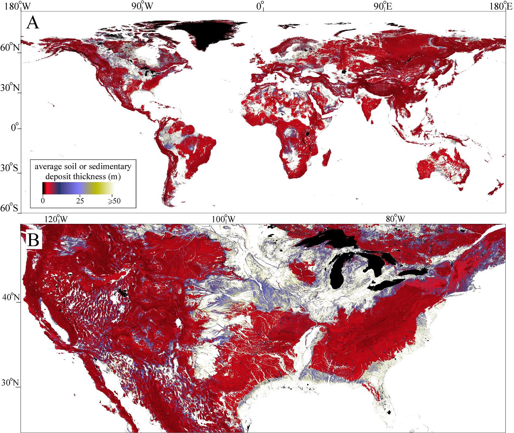
Figure 1. Map of average soil and sedimentary deposit thicknesses within each grid cell. (A) Global, (B) subset of conterminous U.S. (Pelletier et al. 2016).
Citation
Pelletier, J.D., P.D. Broxton, P. Hazenberg, X. Zeng, P.A. Troch, G. Niu, Z.C. Williams, M.A. Brunke, and D. Gochis. 2016. Global 1-km Gridded Thickness of Soil, Regolith, and Sedimentary Deposit Layers. ORNL DAAC, Oak Ridge, Tennessee, USA. http://dx.doi.org/10.3334/ORNLDAAC/1304
Table of Contents
- Data Set Overview
- Data Characteristics
- Application and Derivation
- Quality Assessment
- Data Acquisition, Materials, and Methods
- Data Access
- References
Data Set Overview
Project: Soil Collections
Investigators: Jon D. Pelletier, Patrick D. Broxton, Pieter Hazenberg, Xubin Zeng, Peter A. Troch, Guo-Yue Niu, Zachary Cole Williams, Michael A. Brunke, David Gochis
This data set provides high-resolution estimates of the thickness of the permeable layers above bedrock (soil, regolith, and sedimentary deposits) within a global 30-arcsecond (~ 1 km) grid using the best available data for topography, climate, and geology as input. These data are modeled to represent estimated thicknesses by landform type for the geological present.
The global land surface was partitioned into upland hillslope, upland valley bottom, and lowland landscape components. Models were used to optimize each landform type to estimate the thicknesses of each subsurface layer. On hillslopes, the data were calibrated and validated using independent data sets of measured soil thicknesses from the U.S. and Europe and on lowlands using depth to bedrock observations from groundwater wells in the U.S.
Soil Collections: Soil covers a major portion of the Earth's surface, and is an important natural resource that either directly or indirectly supports most of the planet's life. Soil is a mixture of mineral and organic materials plus air and water. The contents of soil vary by location and are constantly changing. The ORNL DAAC Soil Collections archive contains data on the physical and chemical properties of soils, including: soil carbon and nitrogen, soil water-holding capacity, soil respiration, and soil texture. Most data sets are globally gridded, while a few are of a regional nature.
Data Characteristics
Spatial Coverage
Global (Clipped at -60 degrees south)
Spatial Resolution
30-arcsecond (~1-km) grid cell
Temporal Coverage
These data are modeled to represent estimated thicknesses by landform type for the geological present.
For completeness, the data were given a date range of 1900 to 2015.
Temporal Resolution
One-time estimates
Study Area: (All latitudes and longitudes given in decimal degrees)
|
Site |
Westernmost Longitude | Easternmost Longitude | Northernmost Latitude | Southernmost Latitude |
| Global | -180 | 180 | 90 | -60 |
Data File Information
There are 6 GeoTIFF (.tif) files for high-resolution gridded global estimates of soil and regolith thickness and sedimentary deposit thicknesses above bedrock within each 30-arcsecond (~1 km) grid cell.
File names:
1) upland_hill-slope_regolith_thickness.tif
- A grid (4 byte/float) of the upland regolith (soil plus intact regolith) thickness in meters. This is an experimental product with a high degree of uncertainty as described in Pelletier et al. (2016).
2) upland_hill-slope_soil_thickness.tif
- A grid (4 byte/float) of average upland hillslope soil thickness in meters.
3) hill-slope_valley-bottom.tif
- A grid of the fraction of area within each grid cell composed of hillslopes versus valley bottoms. In most areas, this grid is very close to the value 1.0 because hillslopes occupy the vast majority of area in most landscapes.
4) upland_valley-bottom_and_lowland_sedimentary_deposit_thickness.tif
- A grid of average upland valley bottom and lowland sedimentary deposit thickness in meters.
5) land_cover_mask.tif
- Landcover mask that classifies each grid cell as predominantly ocean, upland, lowland, lake, or perennial ice using values from 0 to 4, respectively.
6) average_soil_and_sedimentary-deposit_thickness.tif
- A grid that averages soil and sedimentary deposit thicknesses in meters for users who want a single thickness value that averages across upland hillslopes and valley bottoms.
User Note for file 6: This is a mosaic or weighted average of grids in file 2 (upland_hill-slope_soil_thickness) and in file 4 (upland_valley-bottom_and_lowland_sedimentary_deposit_thickness). In lowlands, the value in grid 4 is used because there is no significant or systematic difference in sedimentary deposit thickness between hillslopes and valley bottoms. In uplands, the thickness of unconsolidated material varies significantly between hillslopes (where it is at most a few meters) and valley bottoms (where it can be substantially larger than a few meters). In order to derive an average product in uplands that averages appropriately over hillslopes and valley bottoms, it is necessary to weigh the values of grids 2 and 4 in some way. We chose to use both area fraction and the topographic wetness index (TWI) for the weighting, as quantified by equation (7) in Pelletier et al. (2016). This selection was made because, while valley bottoms represent a very small fraction of land area in most cases, all water is routed through valley bottoms as it flows off the landscape. As such, valley bottoms are of greater hydrological significance than their area fraction would suggest. Weighing the thickness of unconsolidated material (soil and sedimentary deposits) by both area and TWI provides one reasonable way to construct a hydrologically relevant estimate for the thickness of unconsolidated material for use in models that do not resolve hillslopes and valley bottoms.
Spatial Data Properties (all files)
Spatial Representation Type: Raster
Number of Bands: 1
Raster Format: GeoTIFF
Number Columns: 43,200
Number Rows: 18,000
Properties specific to each file:
|
File name |
Variable (units) |
Data type |
NoData value |
Minimum valid value |
Maximum valid value |
|
1) upland_hill-slope_regolith_thickness.tif |
regolith thickness (meters) |
Byte |
-1 |
0 |
50 |
|
2) upland_hill-slope_soil_thickness.tif |
soil thickness (meters) |
Float |
-1 |
0 |
4.2 |
|
3) hill-slope_valley-bottom.tif |
area within each pixel composed of hillslopes (fraction) |
Float |
none |
0 |
1 |
|
4) upland_valley-bottom_and_lowland_sedimentary_deposit_thickness.tif |
sedimentary deposit thickness (meters) |
Byte |
-1 |
0 |
50 |
|
5) land_cover_mask.tif |
land cover class (0 - 4) |
Byte |
none |
0 |
4 |
|
6) average_soil_and_sedimentary-deposit_thickness.tif |
soil and sedimentary deposit thicknesses (meters) |
Byte |
-1 |
0 |
50 |
Extent in the data file coordinate system:
Top: 90
Right: 180
Left: -180
Bottom: -60
Application and Derivation
The data will be useful as an input to regional and global hydrological and ecosystems models.
The average_soil_and_sedimentary-deposit_thickness.tif file is for users who prefer to work with a single thickness value within each 30-arcsecond grid cell. We combined the soil thickness values estimated for upland hillslopes together with the values estimated for sedimentary deposit thickness on upland valley bottoms to obtain a single weighted-average value for the relatively porous and unconsolidated material.
Glossary of terms provided by author.
Terms related to subsurface layers/properties:
Thickness: The difference in elevation between the ground surface and the bottom of the various layers considered in the data set. The word “depth” is more commonly used in the literature to refer to this quantity. We use the word thickness because depth refers to a range (i.e. soil depth varies even at any location from 0 to some maximum value) rather than a single value. However, this is a minor distinction and the word thickness should be interpreted to be the same as depth or maximum depth as it is commonly used in the literature.
Paralithic contact: The bottom of the soil layer, where material that can be augered or excavated by hand transitions to weathered bedrock that is mechanically strong and cannot be excavated by hand. Typically denoted as the R horizon by soil scientists.
Soil: Material between the ground surface and the paralithic contact. This is the primary zone that supports life. Typically, much of this layer (A&B horizons) is in transport down the hillslope over geologic time scales. However, soil includes the C horizon (unconsolidated material that is little affected by soil-forming processes and that is not in transport down the slope).
Intact Regolith: The layer between the bottom of the soil and the top of the unweathered bedrock.
Regolith: All material between Earth’s surface and unweathered bedrock. This layer is the sum of the soil and intact regolith layers.
Sedimentary deposits: Unconsolidated material (i.e. material that can be augered or excavated by hand) above bedrock, derived from erosion upslope, in areas susceptible to recent deposition (i.e. upland valley bottoms and lowlands).
Terms related to landscape components and metrics:
The methodology used to create the data set treated upland hillslopes, upland valley bottoms, and lowlands separately for the purpose of estimating soil, regolith, and sedimentary deposit thicknesses.
Uplands: Portions of the landscape that have undergone net erosion over geologic time scales (i.e. ~105 yr and longer). These areas usually have weathered bedrock within a few meters from the surface on hillslopes.
Lowlands: Portions of the landscape that have undergone net deposition over geologic time scales. These areas usually have bedrock tens of meters or more below the surface.
Hillslope: Areas of unconfined overland flow and limited accumulation of sediments.
Valley bottom: Areas where water flow is confined within valley sidewalls or channel banks and where sedimentary deposits are typically a few meters or more in thickness.
Topographic wetness index (TWI): The natural logarithm of the unit contributing area (the contributing area in km2 divided by the grid cell width) divided by the steepest-descent slope.
Quality Assessment
Uncertainty was estimated by computing difference between model prediction and validation data, which included soil depths in Europe and well-derived sedimentary deposit thicknesses in four U.S. states. See Pelletier et al., (2016) for more information.
Data Acquisition, Materials, and Methods
Different methods were applied to estimate the soil, intact regolith, and sedimentary deposit thicknesses on upland hillslopes, upland valley bottoms, and lowlands.
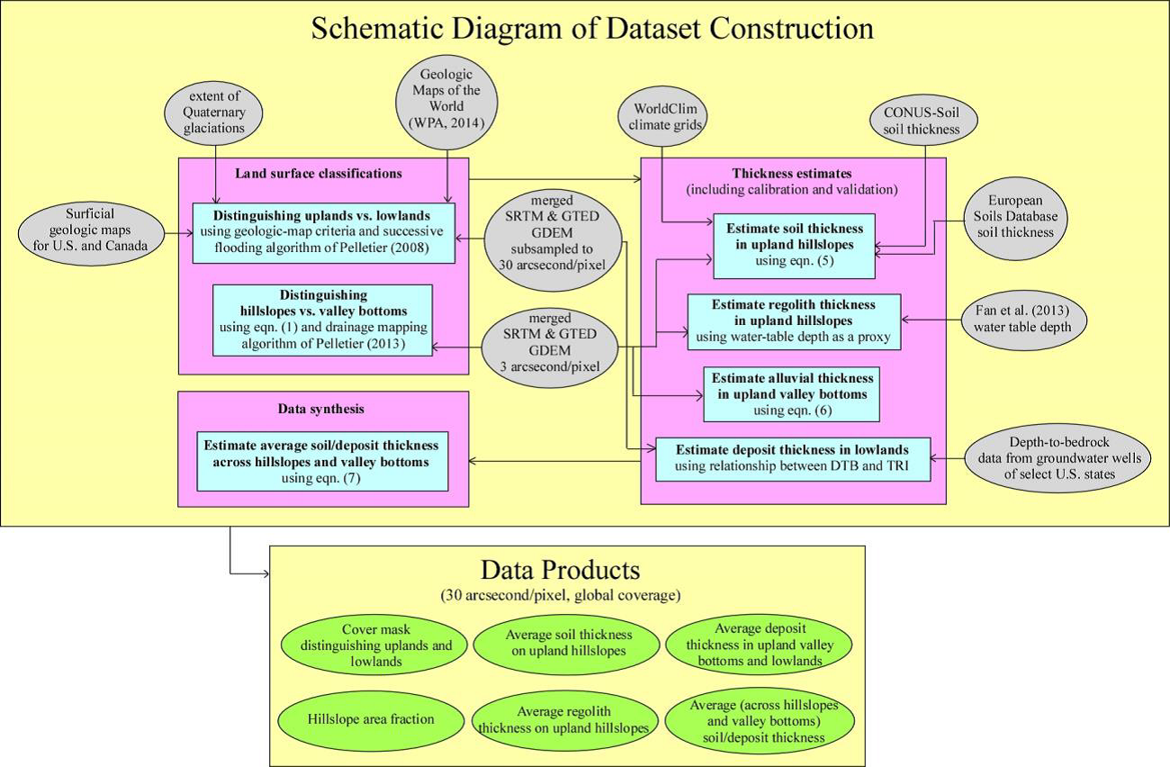
Figure 2. Schematic of data set design construction (Pelletier et al., 2016).
Distinguishing uplands from lowlands
Two types of geologic data, i.e. geologic maps of surficial deposits and geologic maps of the age of the underlying geologic unit, were used to differentiate between uplands and lowlands. The primary source of global geologic information was the collection of digital geologic maps available from the World Petroleum Assessment (WPA, 2014) project of the U.S. Geological Survey (USGS).
The WPA maps were converted from shapefiles to 30-arcsecond raster grids. Separate geologic maps were downloaded for Africa, the Arabian Peninsula, Australia and surrounding islands, Europe, Northeast Asia, Southeast Asia, South Asia, North America, South America, Iran, and the former Soviet Union. Areas mapped as “sedimentary” and “Miocene” or younger were selected from each map to represent lowlands by rasterizing the appropriate polygons. Undifferentiated Cenozoic deposits were also included as lowlands.
For Canada and the USA., surficial geologic maps (Fulton, 1995; Soller et al., 2009) were also used to refine the identification of uplands and lowlands. Areas of continuous surficial deposits were considered lowlands while areas of discontinuous surficial deposits were considered uplands.
The successive flow-routing algorithm of Pelletier (2008) globally at 30-arcsecond resolution was used to identify lowlands not resolved in the geologic maps because additional criteria were needed besides geologic age and type. This iterative algorithm accepts a prescribed runoff depth as input and routes that depth of runoff across the landscape to predict a depth of flow using a combination of Manning’s equation and conservation of discharge. Then, all areas above a threshold depth of flow (including large valleys and their adjacent floodplains) are classified as lowlands if they are not already classified as such using geologic criteria.
However, because the algorithm does not apply to glacial landscapes, in North America lowlands were identified as all areas of continuous glacial deposits in the Soller et al. (2009) and Fulton (1995) maps. In Scandinavia, the extent of former glaciation was defined using Ehlers and Gibbard (2008). A threshold value of the Topographic Ruggedness Index was used to map flatter areas of continuous glacial deposits as lowlands and steeper areas of discontinuous glacial deposits as uplands.
Finally, a combination of the MODIS-based land cover “climatology” (Broxton et al., 2014) and version 2 of the Global Land Cover by National Mapping Organizations (GLCNMO) land cover map (Tateishi et al., 2014) were used to mask out areas beneath oceans, lakes, and perennial ice. Portions of the GLCNMO v2 map were modified within the Great Salt Lake basin because some areas of saline deposits were misclassified as snow/ice in that data set. The Broxton et al. (2014) land-cover climatology data set has a ~500-meter resolution on the MODIS sinusoidal grid. For this project it was regridded to a 30-arcsecond latitude/longitude grid using nearest-neighbor resampling. The GLCNMO v2 land cover map, which has a 15-arcsecond resolution, was similarly regridded to 30-arcsecond.
Distinguishing hillslopes from valley bottoms
The elevation data used is a hybrid of the 3-arcsecond GDEM obtained from measurements of the Shuttle Radar Topography Mission (SRTM; Version 3) (Farr et al., 2007), and the 7.5-arcsecond version of the Global Multi-resolution Terrain Elevation Data 2010 (GMTED2010) produced by the U.S. Geological Survey (USGS) and the National Geospatial-Intelligence Agency (NGA) (Danielson and Gesch, 2011). SRTM data were used where available (from 56 degrees S to 60 degrees N), while GMTED2010 data were used everywhere else. Bilinear interpolation was used to convert the 7.5-arcsecond GMTED2010 product to a 3-arcsecond product.
The method described in Pelletier (2013) was used for drainage network identification that uses only contour curvature (i.e. the curvature of contour lines) to distinguish hillslopes from valley bottoms using a threshold contour curvature of 0.00003 m-1. The algorithm was applied in parallel on the University of Arizona High-Performance-Computing cluster to map hillslopes and valley bottoms at 3-arcsecond resolution, resulting in a seamless global map of valley bottoms and their contributing areas.
Grids distinguishing hillslopes and valley bottoms at 3-arcsecond resolution were used to compute the fraction of area within each 30-arcsecond grid cell comprised of hillslopes. The land area of each 3-arcsecond grid cell mapped as hillslopes was then summed to estimate the fraction of area within each 30-arcsecond grid cell comprised of hillslopes. However, not all of the areas of 3-arcsecond grid cells mapped as valley bottoms are actually valley bottoms. Many small drainage basins have valley bottoms that are ~1–10 m wide that are not resolvable at 3-arcsecond scales. To account for this characteristic, we identified all valley bottoms that were mapped as a single grid cell wide at 3-arcsecond resolution, and estimated the bottom widths, w, of those valleys using a power-law relationship of contributing area, A, measured in units of km2:
w=cAb
where b = 0.4 and c = 3 m are the most representative values based on analyses of small upland fluvial valleys (Whipple, 2004). That is, width is assumed to be 3 m for a drainage basin of contributing area 1 km2 and increases as the 0.4 power of contributing area. While not perfect, this approach is better than the alternative of assuming that all valley bottoms are greater than or equal to ~90 m in width globally.
Estimating soil and regolith thicknesses on upland hillslopes
Soil
The spatial variation of soil thickness in uplands at hillslope-to-watershed scales (Pelletier and Rasmussen, 2009a; Crouvi et al., 2013) was modeled. The CONUS-Soil Data set of Miller and White (1998) was used to calibrate the relationship between upland hillslope soil thickness, mean upland curvature (computed at 3-arcsecond resolution but averaged within each 30-arcsecond grid cell), and mean annual rainfall. The monthly historical mean temperature and precipitation grids of Hijmans et al. (2005) were used to estimate mean annual rainfall globally at 30-arcsecond resolution. High-resolution soil thickness data from the European Soils Database (ESDB) (distributed as part of the Harmonized World Soils Dataset (FAO/IIASA/ISRIC/ISSCAS/JRC, 2012)), were used to validate the upland soil thickness data.
Regolith
The 30-arcsecond equilibrium water table depth gridded data set of Fan et al. (2013) was used to estimate the depth to the permanent water table and hence the thickness of regolith in uplands, following the Rempe and Dietrich (2014) model. However, the Fan et al. (2013) data set as a 30-arcsecond resolution product generally does not resolve many of the low-order valleys in uplands where water table depths often go to zero. To account for this, the water table depths of Fan et al. (2013) were divided by a factor of two to reflect the fact that the average water table depths will generally vary within 30-arcsecond grid cells from a maximum value given by Fan et al. (2013) to zero near valley bottoms.
Estimating sedimentary deposit thickness on upland valley bottoms
The thickness of sedimentary deposits in valley bottoms was predicted using the curvature of the valley bottom and the gradient of the hillslopes flanking the valley to estimate the average thickness of upland valley bottom sedimentary deposits, huv, assuming that the sideslopes project down to a V-shape in the subsurface (a V shape was used because of the predominance of fluvial processes globally):

(the slope gradient on hillslopes divided by the valley-bottom curvature (i.e. the Laplacian))
The equation was applied at the 30-arcsecond resolution using averages of hillslope gradient and valley-bottom curvature within each grid cell computed at 3-arcsecond resolution (Pelletier et al., 2016). Groundwater well data sets were compiled from state geological surveys for much of the conterminous U.S. as a means to validate the predictions.
Estimating sedimentary deposit thickness in lowlands
To estimate the sedimentary deposit thickness in lowlands, a 30-arcsecond grid of Topographic Ruggedness Index (TRI) (Riley et al., 1999) was first generated. TRI is the average elevation difference among a central pixel and its eight neighbors, and thus gives a measure of terrain relief at the grid cell scale. To generate the TRI map, the GDEM data was first regridded to 30-arcsecond resolution (which is the resolution of our soil and sedimentary deposit thickness product). Then, the utility program gdaldem (part of the Geospatial Data Abstraction Library (GDAL)) was used to generate the map of TRI. DTB observations from groundwater wells were used to calibrate a predictive model for DTB as a function of TRI.
Combining soil/sedimentary deposit thicknesses into an averaged product
For lowland areas there is a single estimate of sedimentary deposit thickness for both hillslopes and valley bottoms. For uplands, however, there are two soil/sedimentary deposit thickness values for every pixel: one for hillslopes and one for valley bottoms, plus a fraction of the area of each pixel comprised of hillslopes versus valley bottoms. For users who prefer to work with a single thickness value within each 30-arcsecond pixel, we combined the soil thickness values estimated for upland hillslopes together with the values estimated for sedimentary deposit thickness on upland valley bottoms to obtain a single weighted-average value for the relatively porous and unconsolidated material.
Average soil/sedimentary deposit thickness on uplands, hav, was computed by weighing the thickness values on hillslopes and valley bottoms by both the area fraction and the topographic wetness index (TWI) of hillslopes and valley bottoms (defined as the natural logarithm of the unit contributing area divided by the slope gradient):

(f represents the area fraction of hillslopes versus valley bottoms and the subscript h represents the values for hillslopes and v represents the values for valley bottoms (defined as the natural logarithm of the unit contributing area divided by the slope gradient)
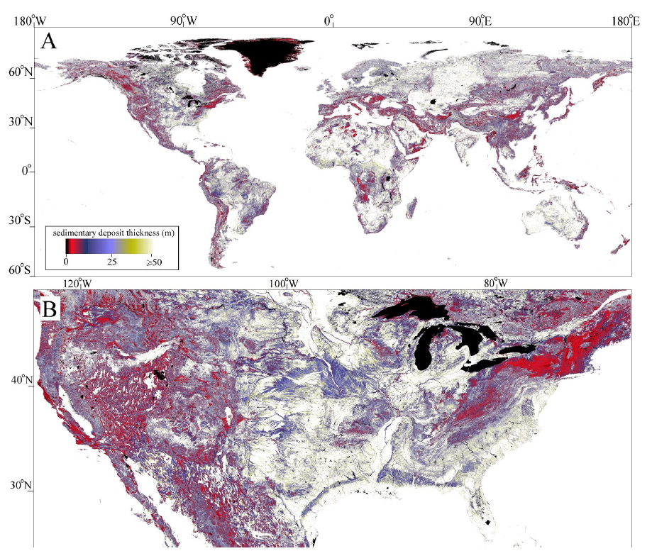
Figure 3. Color maps of average sedimentary deposit thickness in upland valley bottoms and lowlands. (A) Global map, (B) subset of (A) showing the conterminous U.S. (Pelletier et al., 2016).
Data Access
This data is available through the Oak Ridge National Laboratory (ORNL) Distributed Active Archive Center (DAAC).
Global 1-km Gridded Thickness of Soil, Regolith, and Sedimentary Deposit Layers
Contact for Data Center Access Information:
- E-mail: uso@daac.ornl.gov
- Telephone: +1 (865) 241-3952
References
Broxton, P. D., X. Zeng, D. Sulla-Menashe, and P. A. Troch (2014), A Global Land Cover Climatology Using MODIS Data,. J. Appl. Meteor. Climatol., 53, 1593–1605, doi: http://dx.doi.org/10.1175/JAMC-D-13-0270.1
Crouvi, O., J. D. Pelletier, and C. Rasmussen (2013), Predicting the thickness and Aeolian fraction of soils in upland watersheds of the Mojave Desert, Geoderma, 195-196, 94–110,10.1016/j.geoderma.2014.03.003.
Danielson, J. J., and D. B. Gesch (2011), Global Multi-resolution Terrain Elevation Data 2010 (GMTED2010), U.S. Geol. Surv. Open File Report 2011-1073, 26 p.
Ehlers, J., and P. Gibbard (2008), Extent and chronology of Quaternary glaciation, Episodes, 31(2), 211–218.
Fan, Y., H. Li, and G. Miguez-Macho (2013), Global patterns of groundwater table depth, Science, 339, 940–943, doi:10.1126/science.1229881.
FAO/IIASA/ISRIC/ISSCAS/JRC (2012), Harmonized World Soil Dataset (version 1.2), FAO, Rome, Italy and IIASA, Laxenburg, Austria.
Farr, T.G., et al. (2007), The Shuttle Radar Topography Mission, Rev. Geophys., 45, RG2004, doi:10.1029/2005RG000183
Fulton, R. J., (1995) Surficial materials of Canada Matériaux superficiels du Canada, Geological Survey of Canada, "A" Series Map 1880A; 1 sheet, doi:10.4095/205040.
Gochis, D. J., E. R. Vivoni, and C. J. Watts (2010), The Impact of Soil Depth on Land Surface Energy and Water Fluxes in the North American Monsoon Region, J. Arid Environ., 74(5), 564–571, doi:10.1016/j.jaridenv.2009.11.004
Hengl, T., et al. (2014), SoilGrids1km — Global Soil Information Based on Automated Mapping, PLOS One, 9(8), e105992. doi:10.1371/journal.pone.0105992.
Hijmans, R. J., S. E. Cameron, J. L. Parra, P. G. Jones and A. Jarvis (2005), Very high resolution interpolated climate surfaces for global land areas, Inter. J. Climatol., 25, 1965–1978.
Liu, S., Y. Wei, W. M. Post, R. B. Cook, K. Schaefer, and M. M. Thornton (2013), The unified North American soil map and its implication on the soil organic carbon stock in North America, Biogeosciences, 10, 2915–2930, doi:10.5194/bg-10-2915-2013.
Miller, D. A., and R. A. White (1998), A Conterminous United States Multilayer Soil Characteristics Dataset for Regional Climate and Hydrology Modeling, Earth Interactions, 2-002, 1–26.
Pelletier, J. D., P. D. Broxton, P. Hazenberg, X. Zeng, P. A. Troch,G.-Y. Niu, Z. Williams, M. A. Brunke, and D. Gochis (2016), A gridded global data set of soil, immobile regolith, and sedimentary deposit thicknesses for regional and global land surface modeling, J. Adv. Model. Earth Syst.,8, doi:10.1002/2015MS000526
Pelletier, J. D. (2014), The linkage between hillslope vegetation changes and late-Quaternary fluvial-system aggradation in the Mojave Desert revisited, ESurf, 2, 455–468, doi:10.5194/esurf-2-455-2014.
Pelletier, J. D. (2008), Quantitative Modeling of Earth Surface Processes, Cambridge University Press, 304 p.
Pelletier, J. D. (2013), A robust, two-parameter method for the extraction of drainage networks from high-resolution Digital Elevation Models (DEMs): Evaluation and comparison to alternative methods using synthetic and real-world DEMs, Water Resour. Res., 49, 869 doi:10.1029/2012WR012452.
Pelletier, J. D., and C. Rasmussen (2009a), Geomorphically-based predictive mapping of soil thickness in upland watersheds. Water Resour. Res., 45, W09417, doi:10.1029/2008WR007319.
Pelletier, J. D. (2008), Quantitative Modeling of Earth Surface Processes, Cambridge University Press, 304 p.
Rempe, D. M., and W. E. Dietrich (2014), A bottom-up control on fresh-bedrock topography under landscapes, Proc. Nat. Acad. Sci. USA, 111(18), 6576–6581, doi:10.1073/pnas.1404763111.
Riley, S. J., S. D. DeGloria, and R. Elliot (1999), A terrain ruggedness index that quantifies topographic heterogeneity, Inter. J. Sci., 5(1–4), 23–27.
Soil Survey Staff (1999), Soil Taxonomy, Washington, D.C., U.S. Government Printing Office, 869 p. 917
Soller, D. R., M. C. Reheis, C. P. Garrity, and D. R. Van Sistine (2009), Map dataset for surficial materials in the conterminous United States: U.S. Geological Survey Data Series, scale 1:5,000,000, http://pubs.usgs.gov/ds/425/.
Tateishi, R., N. T. Hoan, T. Kobayashi, B. Alsaaideh, G. Tana, and D.X. Phong (2014), J. Geog. Geol., 6(3), doi:10.5539/jgg.v6n3p.
Whipple, K. X. (2004), Bedrock Rivers and the Geomorphology of Active Orogens, Ann. Rev. Earth Planet. Sci., 32, 151–185, 10.1146/annurev.earth.32.101802.120356.
World Petroleum Assessment (WPA) (2014), USGS Energy Resources Program, Digital data downloaded from http://energy.usgs.gov/OilGas/AssessmentsData/WorldPetroleumAssessment/WorldGeologicMaps.aspx